1 Introduction

Diffusion denoising models, first proposed by Sohl-Dickstein et al. (2015); Ho et al. (2020); Ho and Salimans (2022), are generative models that produce data samples through iterative denoising processes. These models achieved superior performance compared to generative adversarial networks (Goodfellow et al., 2020) and became the foundation for many image generation applications such as DALL$\cdot$E 2 (Ramesh et al., 2022), stable diffusion, and Midjourney (Rombach et al., 2022), etc. Given the success in computer vision, diffusion models have been adapted in medical imaging in various fields, including image synthesis (Dorjsembe et al., 2022; Khader et al., 2022), image denoising (Hu et al., 2022), anomaly detection (Wolleb et al., 2022a), classification (Yang et al., 2023), segmentation (Wu et al., 2022; Rahman et al., 2023), and registration (Kim et al., 2022). Among these, segmentation is one of the most foundational tasks in medical imaging and a variety of applications have been explored, including liver CT (Xing et al., 2023), lung CT (Zbinden et al., 2023; Rahman et al., 2023), abdominal CT (Wu et al., 2023; Fu et al., 2023), brain MR (Pinaya et al., 2022a; Wolleb et al., 2022b; Wu et al., 2023; Xing et al., 2023; Bieder et al., 2023), and prostate MR (Fu et al., 2023).

For segmentation tasks, although various model architectures and training strategies  (Wang et al., 2022) have been proposed, U-net equipped with attention mechanisms and trained by supervised learning consistently remains the state-of-the-art model and an important baseline. In comparison, divergent observations have emerged: some studies reported superior performance of diffusion-based segmentation models (Amit et al., 2021; Wu et al., 2022, 2023; Xing et al., 2023), while others observed the opposite trend (Pinaya et al., 2022a; Wolleb et al., 2022b; Kolbeinsson and Mikolajczyk, 2022; Fu et al., 2023). This inconsistency may result from different training schemes, network architectures, and application-specific modifications in comparisons, suggesting that challenges persist in applying diffusion models for image segmentation.

Formally, conditioning on an image, diffusion-based segmentation models operate by progressive denoising, starting with random noise and ultimately yielding the corresponding segmentation masks. In comparison to their non-diffusion counterparts, the necessity of supplementary noisy masks as input leads to increased memory demands that can pose challenges, particularly for processing 3D volumetric medical images. To address this, volume slicing (Wu et al., 2023) or patching (Xing et al., 2023; Bieder et al., 2023) has been used to manage memory limitations. However, diffusion model training still requires considerable computation due to its inherent iterative nature, since the same model needs to learn to denoise masks with varying levels of noise. Consequently, enhancing the diffusion model performance while adhering to a fixed compute budget is of significant importance. Empirically, using the reparametrisation (Kingma et al., 2021), the denoising training task has shifted from noise prediction (Wolleb et al., 2022b; Wu et al., 2022) to mask prediction (Fu et al., 2023; Zbinden et al., 2023) due to the superior performance and faster learning. Furthermore, Fu et al. (2023) highlighted a limitation of diffusion models, noting the misalignment between training and inference procedures, since training samples were generated from ground truth masks. This raises concerns of data leakage as discussed in Chen et al. (2022a). However, there have been limited studies in medical image segmentation that rigorously compare diffusion models with their non-diffusion counterparts and examine diffusion training efficiency.

In this work, we present a substantial extension to the preliminary work (Fu et al., 2023) and focus on an improvement in the diffusion denoising model training strategy that applies to 2D and 3D medical image segmentation in different modalities. First, a novel recycling approach has been introduced. Different from Fu et al. (2023), in the first step during training, the input is completely corrupted by noise instead of a partially corrupted ground truth. This seemingly minor adjustment effectively eliminates the ground truth information from model inputs, which further aligns the training strategy toward inference. The proposed diffusion models can refine or maintain segmentation accuracy throughout the inference process. On the contrary, all other diffusion models demonstrate declining or unstable performance trends. Our research showcases the superior performance of our method compared to established diffusion training strategies (Ho et al., 2020; Chen et al., 2022b; Watson et al., 2023; Fu et al., 2023) for both denoising diffusion probabilistic model-based (Ho et al., 2020) and denoising diffusion implicit model-based (Song et al., 2020a) sampling procedures. We also achieved on-par performance with non-diffusion baselines that had not been observed in the previous study (Fu et al., 2023). Second, we introduce an ensemble model that averages the predicted probabilities from the proposed diffusion-based model and non-diffusion counterpart, resulting in significant improvement to the non-diffusion baseline. Third, we extended the experiments to four large data sets – 2D muscle ultrasound with $3910$ images, 3D abdominal CT with $300$ images, 3D prostate MR with $589$ images, and 3D brain MR with $1251$ images, further demonstrating the robustness of the proposed method against different applications and data types. Lastly, we integrated a Transformer block into our network architecture. This brings our models in line with contemporary state-of-the-art approaches, rendering our findings more pertinent to real-world applications. To mitigate the increased memory consumption resulting from this addition, we employed patch-based training and inference strategies. The JAX-based framework has been released on https://github.com/mathpluscode/ImgX-DiffSeg.

2 Related Works

The diffusion process is a Markov process where data structures are gradually noise-corrupted and eventually destroyed (noising process). A reverse diffusion process (denoising process) can then be learned, where the objective is to gradually recover the data structure. Sohl-Dickstein et al. (2015) first proposed diffusion models which map the disrupted data to a noise distribution. Ho et al. (2020) have shown that such modeling is equivalent to score-matching models, a class of models that estimates the gradient of the log-density (Hyvärinen and Dayan, 2005; Vincent, 2011; Song and Ermon, 2019, 2020). This led to a simplified variational lower bound training objective and a denoising diffusion probabilistic model (DDPM) (Ho et al., 2020). DDPM achieved state-of-the-art performance for unconditional image generation on CIFAR10 at the time. In practice, DDPMs were found suboptimal on log-likelihood estimation and Nichol and Dhariwal (2021) addressed this with a learnable variance schedule, sinusoidal noise schedule, and an importance sampling for time steps. Furthermore, diffusion models were trained with hundreds or thousands of steps, inference with the same number of steps is time-consuming. Therefore, different strategies have been proposed to enable faster sampling. While Nichol and Dhariwal (2021) suggested variance resampling without modifying the probabilistic distribution, Song et al. (2020a) derived a deterministic model, denoising diffusion implicit model (DDIM), which shares the same marginal distribution as DDPM. Liu et al. (2022) further generalized the reverse step of DDIM into an ordinary differential equation and used high-order numerical methods (e.g., Runge-Kutta method) with predicted noise to perform sampling with second-order convergence. Besides, Zheng et al. (2022); Lyu et al. (2022); Guo et al. (2022) accelerated diffusion model training by shortening the noising schedule and only considering a truncated diffusion chain with less noise. These unconditioned denoising diffusion models have been successfully applied in multiple medical imaging applications (Kazerouni et al., 2023), including brain MR image generation (Dorjsembe et al., 2022; Khader et al., 2022), optical coherence tomography denoising (Hu et al., 2022), and chest X-ray pleural effusion detection (Wolleb et al., 2022a).

Guided diffusion models have been developed to generate data in a controllable manner. Song et al. (2020b); Dhariwal and Nichol (2021) used gradients of pre-trained classifiers to bias the sampling process, without modifying the diffusion model training. Ho and Salimans (2022), on the other hand, modified the models to take additional information as input, enabling end-to-end conditional diffusion model training. For medical image synthesis, conditions can be patient biometric information (Pinaya et al., 2022b), genotypes data (Moghadam et al., 2023), or images from different modalities (Saeed et al., 2023). Conditional diffusion models have also been explored for medical image classification (Yang et al., 2023), segmentation (Wu et al., 2022; Rahman et al., 2023), and registration (Kim et al., 2022). Particularly for image segmentation, the diffusion models apply the noising and denoising on the segmentation masks, and the network takes a noisy mask and an image to perform denoising.

In contrast to the continuous spectrum of values found in natural images, image segmentation mask values are categorical and nominal. The Gaussian-based continuous diffusion processes behind DDPM and DDIM cannot be directly applied. Chen et al. (2022b) therefore encoded categories with binary bits and relaxed them to real values for continuous diffusion models. Han et al. (2022); Fu et al. (2023) encoded categories with one-hot embeddings and performed diffusion on scaled values. Li et al. (2022a); Strudel et al. (2022) encoded the discrete data and applied diffusion processes in embedding spaces directly. Alternatively, discrete diffusion models have been proposed to model the transition matrix between categories based on discrete probability distributions, including binomial distribution (Sohl-Dickstein et al., 2015), categorical distribution (Hoogeboom et al., 2021; Austin et al., 2021; Gu et al., 2022), and Bernoulli distribution (Chen et al., 2023). In this work, we follow Fu et al. (2023) to perform diffusion on scaled binary masks.

Originally, DDPM models were trained through noise prediction (Ho et al., 2020), where the loss was calculated between the predicted and sampled noises. Many diffusion-based segmentation models directly adopted this strategy (Wolleb et al., 2022b; Wu et al., 2022). Alternatively, Kingma et al. (2021) derived an equivalent formulation (often known as $\operatorname{\mathbf{x}}_{0}$ reparameterization) of the variational lower bound and simplified the loss to a norm between predicted data and the corresponding ground truth. For segmentation, this is equivalent to predicting the segmentation mask for each time step. Compared to noise prediction, multiple studies found that this mask prediction strategy is more efficient (Fu et al., 2023; Wang et al., 2023; Lai et al., 2023). Furthermore, Chen et al. (2022b) suggested self-conditioning to use these predictions as additional input to improve diffusion models for image synthesis. Self-conditioning contains two steps: the first step predicts a noise-free sample given a noise-corrupted sample only; the second step uses the same timestep and inputs the same noise-corrupted sample, as well as the prediction from the first step. This technique was later adopted for protein design (Watson et al., 2023) with an additional reverse step, where the second step performs denoising in a smaller timestep where the noise level is lower. However, in both cases, the noisy samples are directly derived from the ground truth, which is not available during inference. This risks data leakage during training and empirically leads to overfitting and lack of generalization as discussed in Chen et al. (2022a); Kolbeinsson and Mikolajczyk (2022); Lai et al. (2023). Chen et al. (2022a); Young et al. (2022) addressed this issue by controlling the signal-to-noise ratio so that less information is preserved after noising: Chen et al. (2022a) scaled the mask value ranges to implicitly amplify the noise level, and Young et al. (2022) explicitly varied the scale and standard deviation of the Gaussian noise added to the masks. On the other hand, Kolbeinsson and Mikolajczyk (2022) proposed recursive denoising that iterates through each step during training, without using ground truth as input. However, such a strategy extends the training length by a factor of hundreds or more, making it practically infeasible for larger 3D medical image data sets. Following these studies, Fu et al. (2023) concluded that the lack of generalization in diffusion-based segmentation models is due to the misalignment between training and inference processes. Fu et al. (2023) thus presented a two-step recycling training strategy: the first step ingests a partially noisied sample for mask prediction; the predicted mask is then noise-corrupted again for denoising training. Compared to recursive denoising, this method requires a limited training time increase. This method also resembles PD-DDPM (Guo et al., 2022), where a pre-segmentation is used for noising. However, PD-DDPM requires a separate pre-segmentation network and more device memory, thus not suitable for 3D image segmentation applications.

3 Background

3.1 Denoising Diffusion Probabilistic Model

$$\operatorname{\mathbf{x}}_{T}\autorightleftharpoons{}{}\cdots\autorightleftharpoons{}{}\operatorname{\mathbf{x}}_{t}\autorightleftharpoons{$p_{\theta}(\operatorname{\mathbf{x}}_{t-1}\mid\operatorname{\mathbf{x}}_{t})$}{$q(\operatorname{\mathbf{x}}_{t}\mid\operatorname{\mathbf{x}}_{t-1})$}\operatorname{\mathbf{x}}_{t-1}\autorightleftharpoons{}{}\cdots\autorightleftharpoons{}{}\operatorname{\mathbf{x}}$$

Definition

The denoising diffusion probabilistic models (DDPM) (Ho et al., 2020) consider a forward process (illustrated from right to left in Section 3.1): given a sample $\mathbf{x}_{0}\sim q(\mathbf{x}_{0})$, a noise-corrupted sample $\mathbf{x}_{t}$ follows a multivariate normal distribution at timestep $t\in\{1,\cdots,T\}$, $q(\mathbf{x}_{t}\mid\mathbf{x}_{t-1})=\mathcal{N}(\mathbf{x}_{t};\sqrt{1-\beta_{t}}\mathbf{x}_{t-1},\beta_{t}\mathbf{I})$, where $\beta_{t}\in[0,1]$. As Gaussians are closed under convolution, given $\mathbf{x}_{0}$, $\mathbf{x}_{t}$ can be directly sampled from $\mathbf{x}_{0}$ as follows, $q(\operatorname{\mathbf{x}}_{t}\mid\operatorname{\mathbf{x}}_{0})=\mathcal{N}(\operatorname{\mathbf{x}}_{t};\sqrt{\bar{\alpha}_{t}}\operatorname{\mathbf{x}}_{0},(1-\bar{\alpha}_{t})\mathbf{I})$. Correspondingly, a reverse process (illustrated from left to right in Section 3.1) denoises $\mathbf{x}_{t}$ at each step, for $t\in\{T,\cdots,1\}$, $p_{\theta}(\mathbf{x}_{t-1}\mid\mathbf{x}_{t})=\mathcal{N}(\mathbf{x}_{t-1};\bm{\mu}_{\theta}(\mathbf{x}_{t},t),\sigma_{t}^{2}\mathbf{I})$, with a predicted mean $\bm{\mu}_{\theta}(\mathbf{x}_{t},t)$ and variance $\sigma_{t}^{2}\mathbf{I}$. $\sigma_{t}$ is a pre-defined schedule dependent on timestep $t$. In this work, $\sigma_{t}^{2}=\tilde{\beta}_{t}=\frac{1-\bar{\alpha}_{t-1}}{1-\bar{\alpha}_{t}}\beta_{t}$ with $\alpha_{t}=1-\beta_{t}$ and $\bar{\alpha}_{t}=\prod_{s=1}^{t}\alpha_{s}$. The mean $\bm{\mu}_{\theta}(\mathbf{x}_{t},t)=\frac{\sqrt{\bar{\alpha}_{t-1}}\beta_{t}}{1-\bar{\alpha}_{t}}\hat{\operatorname{\mathbf{x}}}_{0}+\frac{1-\bar{\alpha}_{t-1}}{1-\bar{\alpha}_{t}}\sqrt{\alpha_{t}}\mathbf{x}_{t}$, also know as $\operatorname{\mathbf{x}}_{0}$ parameterization, where $\hat{\operatorname{\mathbf{x}}}_{0}$ is an estimation of $\operatorname{\mathbf{x}}_{0}$ from a learned neural network $\hat{\operatorname{\mathbf{x}}}_{0}=f_{\theta}(\mathbf{x}_{t},t)$.

Training

For each step during training, a noise-corrupted sample $\operatorname{\mathbf{x}}_{t}$ is sampled and input to the neural network $f_{\theta}$ to predict $\operatorname{\mathbf{x}}_{0}$. The network is then trained with loss $L_{\text{denoising}}(\theta)=\operatorname{\mathbb{E}}_{t,\operatorname{\mathbf{x}}_{0},\operatorname{\mathbf{x}}_{t}}L(\operatorname{\mathbf{x}}_{0},\hat{\operatorname{\mathbf{x}}}_{0})$ with $t$ sampled from $1$ to $T$. $L(\cdot,\cdot)$ is a loss function in the space of $\operatorname{\mathbf{x}}$. In this work, importance sampling (Nichol and Dhariwal, 2021) is used for time step $t$, where the weight for $t$ is proportional to $\operatorname{\mathbb{E}}_{\operatorname{\mathbf{x}}_{0},\operatorname{\mathbf{x}}_{t}}L(\operatorname{\mathbf{x}}_{0},\hat{\operatorname{\mathbf{x}}}_{0})$.

$$\operatorname{\mathbf{x}}_{t} \sim\mathcal{N}(\operatorname{\mathbf{x}}_{t};\sqrt{\bar{\alpha}_{t}}\mathbf{x}_{0},(1-\bar{\alpha}_{t})\mathbf{I}), (\text{Sampling})$$(1a)

$$\hat{\mathbf{x}}_{0} =f_{\theta}(t,\mathbf{x}_{t}), (\text{Prediction})$$(1b)

$$L_{\text{denoising}}(\theta) =\operatorname{\mathbb{E}}_{t,\operatorname{\mathbf{x}}_{0},\operatorname{\mathbf{x}}_{t}}L(\operatorname{\mathbf{x}}_{0},\hat{\mathbf{x}}_{0}), (\text{loss calculation})$$(1c)

Inference

At inference time, the denoising starts with a randomly sampled Gaussian noise $\operatorname{\mathbf{x}}_{T}\sim\mathcal{N}(\bm{0},\bm{I})$ and the data is denoised step-by-step for $t=T,\cdots,1$:

$$p_{\theta}(\operatorname{\mathbf{x}}_{t-1}\mid\operatorname{\mathbf{x}}_{t}) =\mathcal{N}(\operatorname{\mathbf{x}}_{t-1};\bm{\mu}_{\theta}(\operatorname{\mathbf{x}}_{t},t),\sigma_{t}^{2}\mathbf{I})$$

$$\bm{\mu}_{\theta}(\operatorname{\mathbf{x}}_{t},t )=\frac{\sqrt{\bar{\alpha}_{t-1}}\beta_{t}}{1-\bar{\alpha}_{t}}\hat{\operatorname{\mathbf{x}}}_{0}+\frac{1-\bar{\alpha}_{t-1}}{1-\bar{\alpha}_{t}}\sqrt{\alpha_{t}}\operatorname{\mathbf{x}}_{t}$$

Optionally, the variance schedule $\beta_{t}$ can be down-sampled to reduce the number of inference steps (Nichol and Dhariwal, 2021). A detailed review of DDPM and the loss has been summarised in Section A and we refer the readers to Sohl-Dickstein et al. (2015); Ho et al. (2020); Nichol and Dhariwal (2021); Kingma et al. (2021) and other literature for in-depth understanding and derivations.

3.2 Diffusion for Segmentation

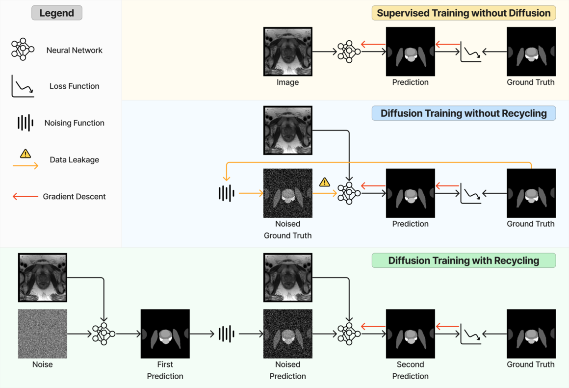
When applying diffusion models for segmentation, noising and denoising are performed on the segmentation masks. The ground-truth binary mask, where channels correspond to classes that include the background, is denoted by $\mathbf{x}_{0}$. For the $i$-th pixel/voxel, the value for the $j$-th channel is in $1$ if it belongs to class $j$ and $-1$ otherwise. The training process (illustrated in LABEL:fig:method_comparison) is similar to Equation 1 except that the segmentation network $f_{\theta}(I,\mathbf{x}_{t},t)$ now takes the image $I$ as an additional input for prediction $\hat{\operatorname{\mathbf{x}}}_{0}$. $L(\cdot,\cdot)$ is a weighted sum of cross entropy and foreground-only Dice loss.

$$\operatorname{\mathbf{x}}_{t} \sim\mathcal{N}(\operatorname{\mathbf{x}}_{t};\sqrt{\bar{\alpha}_{t}}\mathbf{x}_{0},(1-\bar{\alpha}_{t})\mathbf{I}), (\text{Sampling})$$(2a)

$$\hat{\mathbf{x}}_{0} =f_{\theta}(I,t,\mathbf{x}_{t}), (\text{Prediction})$$(2b)

$$L_{\text{denoising}}(\theta) =\operatorname{\mathbb{E}}_{t,\operatorname{\mathbf{x}}_{0},\operatorname{\mathbf{x}}_{t}}L(\operatorname{\mathbf{x}}_{0},\hat{\mathbf{x}}_{0}), (\text{loss calculation})$$(2c)

4 Methods

At each training step, the recycling considers a sampled time step $t<T$ and a data sample $\operatorname{\mathbf{x}}_{0}$. First, a noise-corrupted sample $\operatorname{\mathbf{x}}_{T}$ at time step $T$ is sampled, with $\sqrt{\bar{\alpha}_{T}}\approx 0$. $\operatorname{\mathbf{x}}_{T}$ is fed to the network $f_{\theta}$ to perform a prediction $\hat{\mathbf{x}}_{0}=f_{\theta}(I,T,\mathbf{x}_{T})$. This prediction is then noise-corrupted to generate $\operatorname{\mathbf{x}}_{t}$. A second prediction $\hat{\mathbf{x}}_{0}=f_{\theta}(I,t,\mathbf{x}_{t})$ (overriding the $\hat{\mathbf{x}}_{0}$ for simplicity) is produced and used for loss calculation (see LABEL:fig:method_comparison). Formally, at each timestep $t$, the proposed recycling (denoted as “Diff. rec. $\operatorname{\mathbf{x}}_{T}$”) has the following steps.

$$\operatorname{\mathbf{x}}_{T} \sim\mathcal{N}(\operatorname{\mathbf{x}}_{T};\sqrt{\bar{\alpha}_{T}}\operatorname{\mathbf{x}}_{0},(1-\bar{\alpha}_{T})\mathbf{I}), (\text{rec.}\leavevmode\nobreak\ \operatorname{\mathbf{x}}_{T},\leavevmode\nobreak\ \text{step 1, sampling})$$(3a)

$$\hat{\mathbf{x}}_{0} =\text{StopGradient}(f_{\theta}(I,T,\mathbf{x}_{T})), (\text{rec.}\leavevmode\nobreak\ \operatorname{\mathbf{x}}_{T},\leavevmode\nobreak\ \text{step 1, prediction})$$(3b)

$$\operatorname{\mathbf{x}}_{t} \sim\mathcal{N}(\operatorname{\mathbf{x}}_{t};\sqrt{\bar{\alpha}_{t}}\hat{\mathbf{x}}_{0},(1-\bar{\alpha}_{t})\mathbf{I}), (\text{rec.}\leavevmode\nobreak\ \operatorname{\mathbf{x}}_{T},\leavevmode\nobreak\ \text{step 2, sampling})$$(3c)

$$\hat{\mathbf{x}}_{0} =f_{\theta}(I,t,\mathbf{x}_{t}), (\text{rec.}\leavevmode\nobreak\ \operatorname{\mathbf{x}}_{T},\leavevmode\nobreak\ \text{step 2, prediction})$$(3d)

$$L_{\text{denoising}}(\theta) =\operatorname{\mathbb{E}}_{t,\operatorname{\mathbf{x}}_{0},\operatorname{\mathbf{x}}_{t}}L(\operatorname{\mathbf{x}}_{0},\hat{\mathbf{x}}_{0}), (\text{loss calculation})$$(3e)

In particular, stop gradient is applied to $\hat{\mathbf{x}}_{0}$ in the first step to prevent the gradient calculation across two steps, to reduce training time. Optionally, a model with exponential moving averaged weights can be used, but it requires even more memory. Compared to Equation 2, recycling modification only affects training and does not change network architecture. It is independent of the sampling strategy during inference. Therefore, the DDIM sampler can also be used for inference.

The recycling strategy we propose in this work differs from the one introduced in Fu et al. (2023) (denoted as “Diff. rec. $\operatorname{\mathbf{x}}_{t+1}$”), illustrated in LABEL:fig:method_comparison and the equations below,

$$\operatorname{\mathbf{x}}_{t+1} \sim\mathcal{N}(\operatorname{\mathbf{x}}_{t+1};\sqrt{\bar{\alpha}_{t+1}}\operatorname{\mathbf{x}}_{0},(1-\bar{\alpha}_{t})\mathbf{I}), (\text{rec.}\leavevmode\nobreak\ \operatorname{\mathbf{x}}_{t+1},\leavevmode\nobreak\ \text{step 1, sampling})$$(4a)

$$\hat{\mathbf{x}}_{0} =\text{StopGradient}(f_{\theta}(I,t+1,\mathbf{x}_{t+1})), (\text{rec.}\leavevmode\nobreak\ \operatorname{\mathbf{x}}_{t+1},\leavevmode\nobreak\ \text{step 1, prediction})$$(4b)

$$\operatorname{\mathbf{x}}_{t} \sim\mathcal{N}(\operatorname{\mathbf{x}}_{t};\sqrt{\bar{\alpha}_{t}}\hat{\mathbf{x}}_{0},(1-\bar{\alpha}_{t})\mathbf{I}), (\text{rec.}\leavevmode\nobreak\ \operatorname{\mathbf{x}}_{t+1},\leavevmode\nobreak\ \text{step 2, sampling})$$(4c)

$$\hat{\mathbf{x}}_{0} =f_{\theta}(I,t,\mathbf{x}_{t}), (\text{rec.}\leavevmode\nobreak\ \operatorname{\mathbf{x}}_{t+1},\leavevmode\nobreak\ \text{step 2, prediction})$$(4d)

$$L_{\text{denoising}}(\theta) =\operatorname{\mathbb{E}}_{t,\operatorname{\mathbf{x}}_{0},\operatorname{\mathbf{x}}_{t}}L(\operatorname{\mathbf{x}}_{0},\hat{\mathbf{x}}_{0}), (\text{loss calculation})$$(4e)

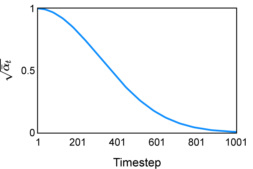
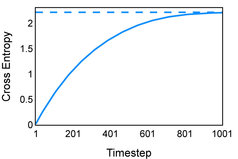
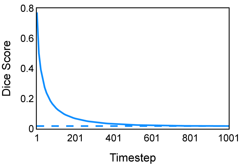
In the new approach (“Diff. rec. $\operatorname{\mathbf{x}}_{T}$”), the first step is consistently executed at the time step $T$ instead of $t+1$ as shown in Equation 3. Compared to $\operatorname{\mathbf{x}}_{t+1}$ in Equation 4, $x_{T}$ is fully noised and contains even less ground truth information during the initial step. Specifically, for a given time step $t$, $\operatorname{\mathbf{x}}_{t}\sim\mathcal{N}(\operatorname{\mathbf{x}}_{t};\sqrt{\bar{\alpha}_{t}}\operatorname{\mathbf{x}}_{0},(1-\bar{\alpha}_{t})\mathbf{I})$, which can be reparameterized as $\operatorname{\mathbf{x}}_{t}=\sqrt{\bar{\alpha}_{t}}\operatorname{\mathbf{x}}_{0}+\sqrt{1-\bar{\alpha}_{t}}\operatorname{\bm{\epsilon}}_{t}$ with $\operatorname{\bm{\epsilon}}_{t}\sim\mathcal{N}(\mathbf{0},\mathbf{I})$ and $\bar{\alpha}_{t}=\prod_{s=1}^{t}\alpha_{s}$. In this work, $\alpha_{t}$ is a monotonically decreasing noise schedule ranging from $0.999$ to $0.98$ for $t=1$ to $T$. Correspondingly, $\sqrt{\bar{\alpha}_{t}}$ monotonically decreases from $0.99995$ to $0.00632$. $\operatorname{\mathbf{x}}_{T}=\sqrt{\bar{\alpha}_{T}}\operatorname{\mathbf{x}}_{0}+\sqrt{1-\bar{\alpha}_{T}}\operatorname{\bm{\epsilon}}_{T}$ with $\sqrt{\bar{\alpha}_{T}}=0.00632$ can be considered to contain almost no ground truth information. The information can also be empirically measured by cross entropy and Dice score, and an example is presented in Figure 2 in Section D. This seemingly minor modification removes the ground truth information from model inputs, essentially reducing the risk of data leakage and training overfitting. This adaptation guides the model to learn the denoising task based on its initial prediction, rather than ground truth. Consequently, the model can effectively denoise and refine the provided noisy mask, ultimately predicting the ground truth.

Recycling also differs from the self-conditioning methods proposed in Chen et al. (2022b) (“Diff. sc. $\operatorname{\mathbf{x}}_{t}$”) and Watson et al. (2023) (“Diff. sc. $\operatorname{\mathbf{x}}_{t+1}$”). Although self-conditioning also requests two forward loops during training, it differs from recycling in multiple aspects. First, noisy samples in self-conditioning are always generated based on ground truth $\operatorname{\mathbf{x}}_{0}$, while the second forward step of recycling does not rely on ground truth for noisy sample generation. Second, self-conditioning provides an additional input $\hat{\operatorname{\mathbf{x}}}_{0}$, while recycling does not. Lastly, in self-conditioning, $\hat{\operatorname{\mathbf{x}}}_{0}$ is replaced by zeros with $50\%$ probabilities, while recycling is applied constantly. The training strategy has been detailed in LABEL:fig:method_comparison and Section C. For further details, we refer the reader to the reference papers (Chen et al., 2022b; Watson et al., 2023).

5 Experiments

5.1 Experiment Setting

A range of experiments have been performed in four data sets (Section 5.2) to evaluate the proposed method and the trained models from different aspects.

5.1.1 Diffusion Training Strategy Comparison

First, the proposed recycling training strategy (“Diff. rec. $\operatorname{\mathbf{x}}_{T}$”) was compared with standard diffusion models (“Diff.”) and other diffusion training strategies that require two forward steps to evaluate the training efficiency with identical network architectures and compute budget. The compared diffusion training strategies include the previously proposed recycling method Fu et al. (2023) (“Diff. rec. $\operatorname{\mathbf{x}}_{t+1}$”) and two self-conditioning techniques from Chen et al. (2022b) (“Diff. sc. $\operatorname{\mathbf{x}}_{t}$”) and Watson et al. (2023) (“Diff. sc. $\operatorname{\mathbf{x}}_{t+1}$”). For each trained model using a different strategy, both DDPM and DDIM samplers were evaluated. Importantly, the predictions at each inference step were assessed to study the variation of performance along the inference process.

5.1.2 Comparison to Non-diffusion Models

The proposed methods were compared with non-diffusion-based models using identical architectures and the same compute budget. An ensemble model was also evaluated, where the predicted probabilities from the diffusion model and non-diffusion model were averaged. Models’ segmentation accuracy was assessed with different granularities: per foreground class or averaged across foreground classes. Balnd-altmann plots were used to analyze the differences between models.

5.1.3 Ablation Studies for Recycling

Ablation studies were performed, including assessing the performance with different lengths of inference and evaluating the stochasticity across different seeds during inference. Compared to the previous work (Fu et al., 2023), the effectiveness of the Transformer architecture and the change of training noise schedule was evaluated.

5.1.4 Evaluation Metrics

Different methods were evaluated using binary Dice score (DS) and $95\%$ Hausdorff distance (HD), averaging over foreground classes on the test sets. Dice score is reported in percentage, between $0\%$ and $100\%$. For Hausdorff distance, the values are in mm for 3D volumes and pixels for 2D images. Paired Student’s t-tests with a significance level of $\alpha=0.05$ were performed on the Dice score to test statistical significance between model performance.

5.2 Data

5.2.1 Muscle Ultrasound

The data set (Marzola et al., 2021) provides $3910$ labeled transverse musculoskeletal ultrasound images, which were split into $2531$, $666$, and $713$ images for training, validation, and test sets, respectively. Images had the shape $480\times 512$. The predicted masks were post-processed, following Marzola et al. (2021). After filling the holes, multiple morphological operations were performed, including an erosion with a disk of radius 3 pixels, a dilation with a disk of radius 5 pixels, and an opening with a disk of radius 10 pixels. Afterward, only the largest connected component was preserved if the second largest structure was smaller than 75% of the largest one; otherwise, the most superficial (i.e., towards the top of the image) one between the two largest components was preserved. Finally, holes were filled if there were any.

5.2.2 Abdominal CT (AMOS)

The data set (Ji et al., 2022) provides $200$ and $100$ CT image-mask pairs for $15$ abdominal organs in training and validation sets. The validation set was randomly split into non-overlapping validation and test sets, with $10$ and $90$ images, respectively. The images were first resampled with a voxel dimension of $1.5\times 1.5\times 5.0$ (mm). HU values were clipped to $[-991,362]$ and images were normalized so that the intensity had zero mean and unit variance. Lastly, images were center-cropped to shape $192\times 128\times 128$. During training, the patch size was $128\times 128\times 128$. During inference, the overlap between patches is $64\times 0\times 0$, and the predictions on the overlap were averaged.

5.2.3 Prostate MR

The data set (Li et al., 2022b) contains $589$ T2-weighted image-mask pairs for $8$ anatomical structures from $7$ institutions. The images were randomly split into non-overlapping training, validation, and test sets, with $411$, $14$, and $164$ images in each split, respectively. The validation split has two images of each institution. The images were resampled with a voxel dimension of $0.75\times 0.75\times 2.5$ (mm). Afterward, images were normalized so that the intensity had zero mean and unit variance. Lastly, the images were center-cropped to shape $256\times 256\times 48$. During training, the patch size was $256\times 256\times 32$. During inference, the overlap between patches was $0\times 0\times 16$, and the predictions on the overlap were averaged.

5.2.4 Brain MR (BraTS 2021)

The data set (Baid et al., 2021) provides $1251$MR segmented mpMRI scans for brain tumour. The data set was randomly split into non-overlapping training, validation, and test sets, with $938$, $31$, and $282$ samples, respectively. The whole tumor mask was generated as foreground class, including GD-enhancing tumor, the peritumoral edematous/invaded tissue, and the necrotic tumor core. Therefore, the task was a binary segmentation. Four modalities are available, including T1-weighted (T1), post-contrast T1-weighted (T1Gd), T2-weighted (T2), and T2 Fluid Attenuated Inversion Recovery (T2-FLAIR). The voxel dimension was $1.0\times 1.0\times 1.0$ (mm). Images were firstly normalized so that the intensity has zero mean and unit variance. Lastly, images were center-cropped to shape $179\times 219\times 155$ to remove the common background. During training, the patch size was $128\times 128\times 128$. During inference, the overlap between patches was $77\times 37\times 101$, and the predictions on the overlap were averaged.

5.3 Implementation Details

Figure 1: Unet architecture for diffusion and non-diffusion models. The inputs are concatenated when a noisy mask (from diffusion models) or predicted mask (from self-conditioning) is provided. The tensor is enriched with convolution (time-conditioned for diffusion models) and down-sampling layers, then passed into a Transformer with positional encoding, the output is then enriched with convolution and up-sampling layers, and finally, prediction is performed with an additional $1\times 1$ convolutional layer. “Pred.” stands for predicted.

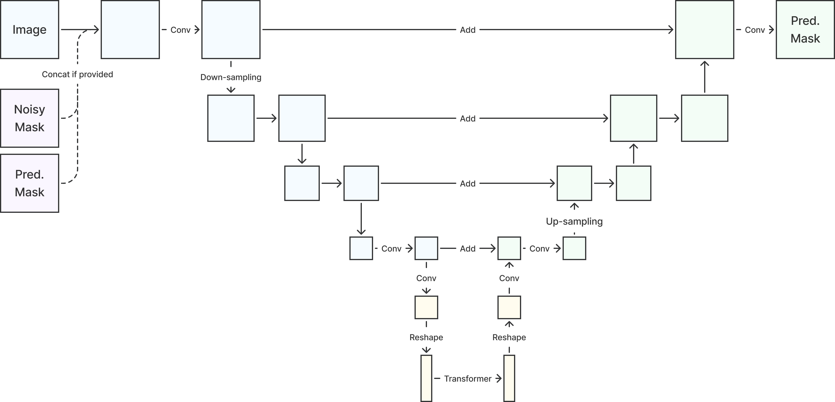
2D and 3D U-net variants with attention mechanisms were used for benchmarking the reference performance from cross-data-set non-diffusion models. The architecture is illustrated in Figure 1. U-nets have four layers with $32$, $64$, $128$, and $256$ channels, respectively. The numbers of learnable parameters are summarized in Table 7 in Section E. For diffusion-based models, the noise-corrupted masks were concatenated. Time was encoded using sinusoidal positional embedding (Rombach et al., 2022) and used in the convolution layers.

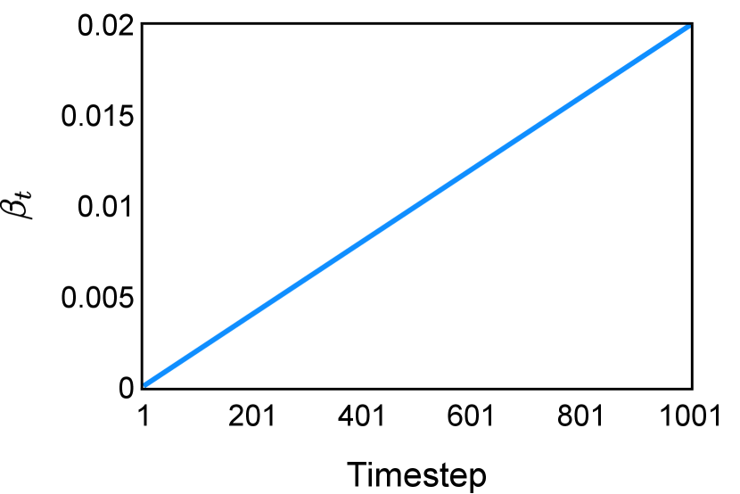
For denoising training, a linear $\beta$ schedule between $0.0001$ and $0.02$ was used for $T=1001$ (illustrated in Figure 2 in Section D). The segmentation-specific loss function is a weighted sum of cross-entropy and foreground-only Dice loss, with weight $20$ and $1$ respectively (Kirillov et al., 2023). Random rotation, translation, and scaling were adopted for data augmentation during training. Training hyper-parameters are listed in Table 6 in Section E. Hyper-parameters were configured empirically without extensive tuning.

Models were trained once and checkpoints were saved every $500$ step. The checkpoint that had the best mean binary Dice score (without background class) in the validation set was used for the testing. For DDIM, the training was the same as DDPM while both validation and testing were performed using DDIM. The variance schedule was down-sampled to $5$ steps (Nichol and Dhariwal, 2021). Experiments were carried out using bfloat16 mixed precision on TPU v3-8, which has $16\times 8$ GB device memory. However, each device has only 16 GB memory, meaning that the model and data have to fit into $16$ GB memory. The JAX-based framework has been released on https://github.com/mathpluscode/ImgX-DiffSeg.

6 Results and Discussion

6.1 Diffusion Training Strategy Comparison

Table 1: Diffusion training strategies comparison. “Diff.” represents standard diffusion. “Diff. sc. $\operatorname{\mathbf{x}}_{t}$” and “Diff. sc. $\operatorname{\mathbf{x}}_{t+1}$” represents self-conditioning from Chen et al. (2022b) and Watson et al. (2023), respectively. “Diff. rec. $\operatorname{\mathbf{x}}_{t+1}$” and “Diff. rec. $\operatorname{\mathbf{x}}_{T}$” represents recycling from Fu et al. (2023) and the proposed recycling in this work, respectively. The best results are in bold and underline indicates the difference to the second best is significant with p-value $<0.05$.

Method	DDPM		DDIM
	DS $\uparrow$	HD $\downarrow$	DS $\uparrow$	HD $\downarrow$
Diff.	86.60 $\pm$ 12.38	41.11 $\pm$ 35.48	86.18 $\pm$ 12.41	42.31 $\pm$ 35.82
Diff. sc. $\operatorname{\mathbf{x}}_{t}$	86.35 $\pm$ 14.14	40.42 $\pm$ 37.53	85.96 $\pm$ 13.78	42.00 $\pm$ 36.76
Diff. sc. $\operatorname{\mathbf{x}}_{t+1}$	87.14 $\pm$ 11.48	39.24 $\pm$ 32.83	86.30 $\pm$ 11.49	41.89 $\pm$ 32.72
Diff. rec. $\operatorname{\mathbf{x}}_{t+1}$	87.44 $\pm$ 12.39	39.68 $\pm$ 36.21	87.43 $\pm$ 12.25	39.82 $\pm$ 35.39
Diff. rec. $\operatorname{\mathbf{x}}_{T}$	88.23 $\pm$ 11.69	35.37 $\pm$ 31.79	88.21 $\pm$ 11.70	35.52 $\pm$ 31.91

(a) Muscle Ultrasound

Method	DDPM		DDIM
	DS $\uparrow$	HD $\downarrow$	DS $\uparrow$	HD $\downarrow$
Diff.	85.25 $\pm$ 5.36	7.12 $\pm$ 3.83	85.59 $\pm$ 5.24	7.13 $\pm$ 3.98
Diff. sc. $\operatorname{\mathbf{x}}_{t}$	86.04 $\pm$ 5.12	7.06 $\pm$ 4.20	85.50 $\pm$ 5.14	7.21 $\pm$ 4.16
Diff. sc. $\operatorname{\mathbf{x}}_{t+1}$	85.86 $\pm$ 5.27	6.98 $\pm$ 3.54	85.25 $\pm$ 5.42	7.28 $\pm$ 3.72
Diff. rec. $\operatorname{\mathbf{x}}_{t+1}$	86.48 $\pm$ 5.24	6.69 $\pm$ 4.59	86.35 $\pm$ 5.31	6.75 $\pm$ 4.55
Diff. rec. $\operatorname{\mathbf{x}}_{T}$	87.45 $\pm$ 5.43	6.56 $\pm$ 5.44	87.45 $\pm$ 5.43	6.55 $\pm$ 5.43

(b) Abdominal CT

Method	DDPM		DDIM
	DS $\uparrow$	HD $\downarrow$	DS $\uparrow$	HD $\downarrow$
Diff.	83.61 $\pm$ 4.87	5.10 $\pm$ 2.40	83.11 $\pm$ 4.81	5.00 $\pm$ 2.35
Diff. sc. $\operatorname{\mathbf{x}}_{t}$	83.47 $\pm$ 4.85	5.17 $\pm$ 2.65	82.49 $\pm$ 4.88	5.42 $\pm$ 2.70
Diff. sc. $\operatorname{\mathbf{x}}_{t+1}$	83.97 $\pm$ 4.85	4.93 $\pm$ 2.66	83.00 $\pm$ 4.89	5.10 $\pm$ 2.64
Diff. rec. $\operatorname{\mathbf{x}}_{t+1}$	84.29 $\pm$ 5.12	4.59 $\pm$ 2.21	84.21 $\pm$ 4.89	4.96 $\pm$ 2.92
Diff. rec. $\operatorname{\mathbf{x}}_{T}$	85.54 $\pm$ 5.20	4.40 $\pm$ 1.96	85.54 $\pm$ 5.20	4.41 $\pm$ 1.96

(c) Prostate MR

Method	DDPM		DDIM
	DS $\uparrow$	HD $\downarrow$	DS $\uparrow$	HD $\downarrow$
Diff.	90.29 $\pm$ 12.98	8.46 $\pm$ 15.55	89.94 $\pm$ 13.00	8.55 $\pm$ 15.50
Diff. sc. $\operatorname{\mathbf{x}}_{t}$	90.12 $\pm$ 12.39	9.55 $\pm$ 17.18	89.73 $\pm$ 12.61	9.67 $\pm$ 16.86
Diff. sc. $\operatorname{\mathbf{x}}_{t+1}$	89.11 $\pm$ 14.70	9.63 $\pm$ 17.47	88.75 $\pm$ 14.77	9.62 $\pm$ 16.97
Diff. rec. $\operatorname{\mathbf{x}}_{t+1}$	86.97 $\pm$ 10.94	9.83 $\pm$ 12.62	84.76 $\pm$ 13.42	12.52 $\pm$ 15.55
Diff. rec. $\operatorname{\mathbf{x}}_{T}$	92.29 $\pm$ 8.55	7.03 $\pm$ 13.48	92.29 $\pm$ 8.55	7.03 $\pm$ 13.48

(d) Brain MR

Our proposed recycling method (Diff. rec. $\operatorname{\mathbf{x}}_{T}$) achieved mean Dice scores of $88.23\%$, $87.45\%$, $85.54\%$, and $92.29\%$ on muscle ultrasound, abdominal CT, prostate MR, and brain MR data sets, respectively. These scores marked absolute improvements of $1.63\%$, $2.20\%$, $1.93\%$, and $2.00\%$ over standard diffusion models, respectively. The relative improvements are $1.88\%$, $2.58\%$, $2.31\%$, and $2.22\%$ respectively. Impressively, this novel strategy consistently outperformed the other three training approaches in terms of both Dice score and Hausdorff distance. The observed differences were significant for all data sets in terms of Dice score ($p=0.003$ for muscle ultrasound and $p<0.001$ for other data sets). These findings held for both the DDPM and the DDIM samplers, underscoring the wide applicability of the proposed training strategy.

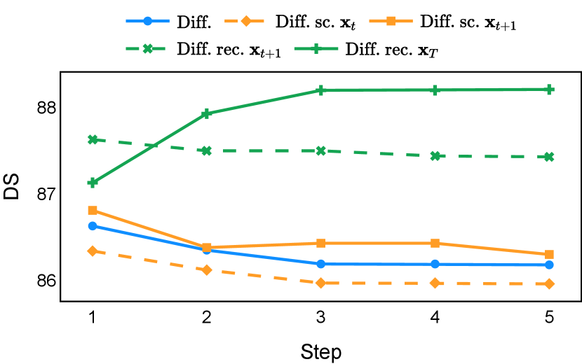
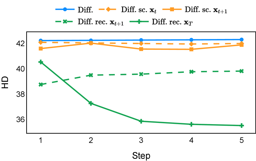
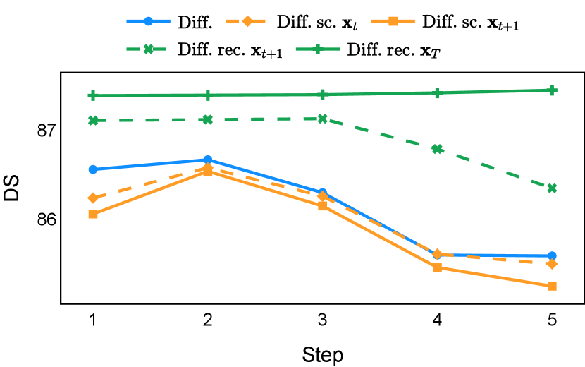
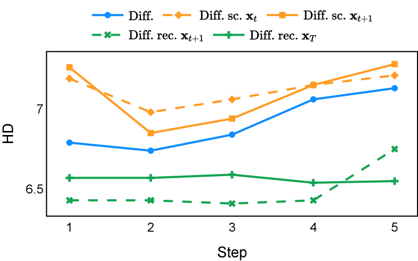
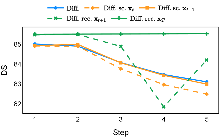
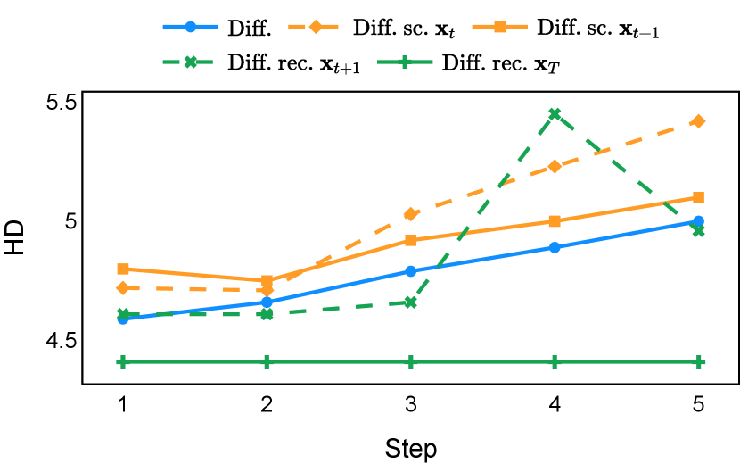
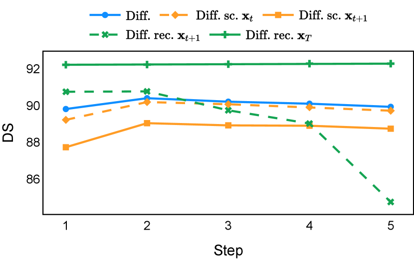
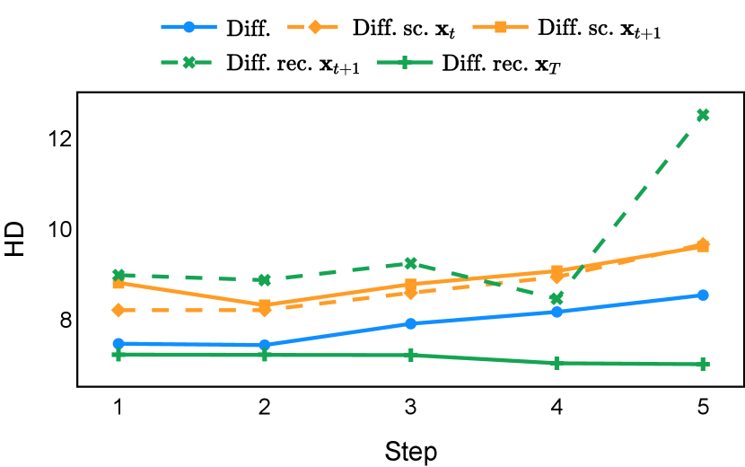
As depicted in Figure 3 in Section F.1, standard diffusion models often produce segmentation masks in the last step that are less accurate than the initial prediction. Similar challenges were observed with self-conditioning strategies and previously proposed recycling methods. The newly introduced recycling method was the only approach that improved initial segmentation predictions for more than half of the test images. Moreover, the average performance per step has been visualized in LABEL:fig:per_step_ddpm, where diffusion models frequently exhibit gradually declining or unstable performance during inference, in terms of both Dice score and Hausdorff distance. It is interesting to observe that often the optimal prediction emerges not at the final step but rather at an intermediate stage. This has been observed in all diffusion models except the newly proposed diffusion model with the innovative recycling method. In the latter case, the quality of segmentation consistently improved or remained stable throughout the inference process, distinguishing it from the observed trend. A qualitative comparison on an example muscle ultrasound image has been illustrated in LABEL:fig:comparison_muscle_ultrasound, where the proposed diffusion model was able to refine the segmentation mask progressively. Similar observations have been noted with the DDIM sampler as well, as shown in Figure 4 and Figure 5. This finding aligns with the discussions from Kolbeinsson and Mikolajczyk (2022); Lai et al. (2023) that the diffusion-based segmentation model performance is strongly influenced by the prediction of the initial step. For self-conditioning or the previously proposed recycling, the denoising training relies on the ground truth to varying degrees therefore the diffusion models are trained with ground truth-like initial predictions. However, no ground truth is available during inference, and the distributions of initial predictions from the trained models are dissimilar from ground truths. This results in an out-of-sample inference and therefore a declining performance. In contrast, the proposed method ingests model predictions for both the training and inference phases without the bias toward ground truth. These observations reaffirm the importance and benefits of harmonizing the training and inference processes. This alignment is crucial to mitigate data leakage, prevent overfitting, and help generalization.

6.2 Comparison to Non-diffusion Models

Table 2: Segmentation performance comparison to non-diffusion models. “No diff.” represents non-diffusion model. “Diff. rec. $\operatorname{\mathbf{x}}_{T}$” represents the diffusion model with proposed recycling. “Ensemble” represents the model averaging the probabilities from “No diff.” and “Diff. rec. $\operatorname{\mathbf{x}}_{T}$”. The inference sampler is DDPM. The best results are in bold and underline indicates the difference to non-diffusion model is significant with p-value < $0.05$.

Data Set	Method	DS $\uparrow$	HD $\downarrow$
Muscle Ultrasound	No diff.	88.15 $\pm$ 10.77	36.86 $\pm$ 30.04
	Diff. rec. $\operatorname{\mathbf{x}}_{T}$	88.23 $\pm$ 11.69	35.37 $\pm$ 31.79
	Ensemble	88.88 $\pm$ 10.59	34.01 $\pm$ 28.75
Abdominal CT	No diff.	87.59 $\pm$ 5.10	6.36 $\pm$ 3.86
	Diff. rec. $\operatorname{\mathbf{x}}_{T}$	87.45 $\pm$ 5.43	6.56 $\pm$ 5.44
	Ensemble	88.29 $\pm$ 5.21	5.60 $\pm$ 3.13
Prostate MR	No diff.	85.22 $\pm$ 5.18	4.62 $\pm$ 2.37
	Diff. rec. $\operatorname{\mathbf{x}}_{T}$	85.54 $\pm$ 5.20	4.40 $\pm$ 1.96
	Ensemble	85.95 $\pm$ 5.12	4.32 $\pm$ 2.01
Brain MR	No diff.	92.43 $\pm$ 9.10	5.20 $\pm$ 9.56
	Diff. rec. $\operatorname{\mathbf{x}}_{T}$	92.29 $\pm$ 8.55	7.03 $\pm$ 13.48
	Ensemble	92.67 $\pm$ 8.60	5.03 $\pm$ 8.41

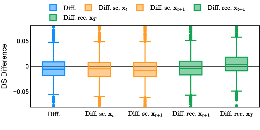
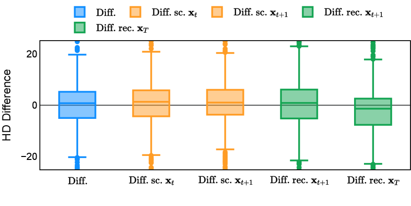
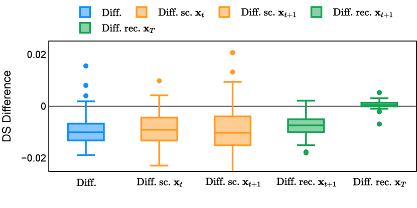
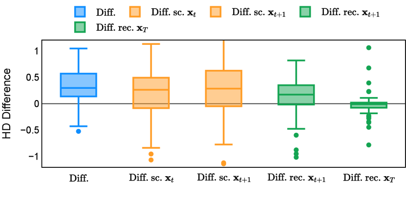
The proposed diffusion models (“Diff. rec. $\operatorname{\mathbf{x}}_{T}$”) were compared with their non-diffusion counterparts (“No diff.”), where models with identical architectures were trained under the same scheme with the same compute budget. This provides a fair comparison without application-specific adjustments. For diffusion models, the performance with DDPM was selected. As shown in Table 2, The diffusion models yielded similar performance across all data sets. The difference in Dice score is not significant for muscle ultrasound, abdominal CT, and brain MR, but the diffusion model had a higher Dice score for prostate MR ($p=0.001$). Furthermore, LABEL:fig:diff_vs_nodiff shows that the proposed diffusion model achieved a higher Dice score on more than $50\%$ samples for muscle ultrasound, abdominal CT, and prostate MR data sets. To the best of our knowledge, this is the first time that diffusion models achieved comparable performance against standard non-diffusion-based models with the same architecture and compute budget.

By ensembling these two models via averaging the probabilities, we achieved mean Dice scores of $88.88\%$, $88.29\%$, $85.95\%$, and $92.67\%$ on muscle ultrasound, abdominal CT, prostate MR, and brain MR data sets, respectively. The improvements in Dice score were significant across all four data sets ($p=0.037$ for brain MR and $p<0.001$ for other data sets). Especially, LABEL:fig:diff_vs_nodiff shows that the ensemble model reached a higher Dice score compared to non-diffusion models on $70.83\%$, $91.11\%$, $89.02\%$, and $64.54\%$ samples in the test set for muscle ultrasound, abdominal CT, prostate MR data and brain MR, respectively. These scores marked an absolute increase of $19.36\%$, $40.00\%$, $28.04\%$, and $19.44\%$ compared to the diffusion model alone. Moreover, Abdominal CT and prostate MR are two data sets with multiple classes and their per-class segmentation performances are summarised in Table 8 and Table 9 in Section F.1, respectively. Upon comparing diffusion models and non-diffusion models, neither consistently outperformed the other across all classes. However, the ensemble model reached the best performance across all classes and the improvement of Dice score is significant for 13 out of 15 classes in Abdominal CT data and all classes in prostate MR data (all p-values $<=0.01$, excluding Spleen $p=0.06$ and Gall bladder $p=0.876$). Multiple examples have also been visualized in LABEL:fig:3d and LABEL:fig:brain_mr_3d for the segmentation error.

We highlight that the value of the competitive performance from alternative methods, in particular a different class of generative model-based approaches, is beyond the replacement of current segmentation algorithms for specific potential applications. Our results demonstrate a consistent improvement by combining diffusion and non-diffusion models across applications, even when they yielded a similar performance individually. This is one of the possible potential uses of the proposed improved diffusion models in addition to the well-established non-diffusion baseline. Future research could explore application-specific tuning for further performance improvements.

6.3 Ablation Studies

6.3.1 Number of sampling steps

Table 3: Diffusion with different number of sampling steps. Sampler is DDPM. Diffusion models were trained using the proposed recycling method (Diff. rec. $\operatorname{\mathbf{x}}_{T}$). OOM indicates that out of memory errors were encountered. Best results are in bold.

Data Set	# Sampling Steps	Dice Score	Hausdorff Distance
Muscle Ultrasound	2	88.01 $\pm$ 12.07	36.55 $\pm$ 32.66
	5	88.23 $\pm$ 11.69	35.37 $\pm$ 31.79
	11	88.30 $\pm$ 11.29	35.25 $\pm$ 30.64
Abdominal CT	2	87.44 $\pm$ 5.43	6.56 $\pm$ 5.42
	5	87.45 $\pm$ 5.43	6.56 $\pm$ 5.44
	11	OOM	OOM
Prostate MR	2	85.54 $\pm$ 5.19	4.40 $\pm$ 1.96
	5	85.54 $\pm$ 5.20	4.40 $\pm$ 1.96
	11	85.54 $\pm$ 5.20	4.40 $\pm$ 1.96
Brain MR	2	92.29 $\pm$ 8.54	7.03 $\pm$ 13.47
	5	92.29 $\pm$ 8.55	7.03 $\pm$ 13.48
	11	92.29 $\pm$ 8.57	7.02 $\pm$ 13.48

Diffusion models were trained using a thousand steps, yet employing the same number of steps for inference can be cost-prohibitive, particularly for processing 3D image volumes. As a result, practical inference commonly utilizes a condensed schedule with a limited number of steps. While this approach reduces computational expenses, the resulting sample quality might be compromised. An ablation study of the numbers of timesteps during inference has therefore been performed across data sets with the proposed recycling-based diffusion model. DDPM sampler was used. The results have been summarised in Table 3. Notably, increasing the number of steps yielded a higher Dice score for the muscle ultrasound dataset but the difference is not significant ($p>=0.05$). For prostate MR and brain MR data sets, the models maintained almost the same performance regardless of the inference length ($p>=0.05$). Given that longer inference times and increased device memory usage are associated with more timesteps (e.g. out-of-memory errors were encountered with Abdominal CT at 11 steps), the trade-off between computational resources and performance suggests that a five-step sampling schedule provides the optimal balance.

6.3.2 Inference Variance

Table 4: Diffusion model performance across different inference seeds. For each sample, the maximum difference ($\Delta$) across five random seeds is calculated. The average across all samples is reported.

Data Set	Mean $\Delta$ Dice Score
	Step 1	Step 2	Step 3	Step 4	Step 5
Muscle Ultrasound	0.0212	0.0165	0.0122	0.0081	0.0051
Abdominal CT	0.0009	0.0010	0.0009	0.0008	0.0004
Prostate MR	0.0004	0.0004	0.0004	0.0004	0.0002
Brain MR	0.0005	0.0005	0.0005	0.0003	0.0001
Data Set	Mean $\Delta$ Hausdorff Distance
	Step 1	Step 2	Step 3	Step 4	Step 5
Muscle Ultrasound	10.0582	7.0020	4.7440	3.1758	1.8164
Abdominal CT	0.1481	0.1339	0.1221	0.0751	0.0673
Prostate MR	0.0447	0.0426	0.0499	0.0431	0.0209
Brain MR	0.0758	0.0779	0.0678	0.0616	0.0197

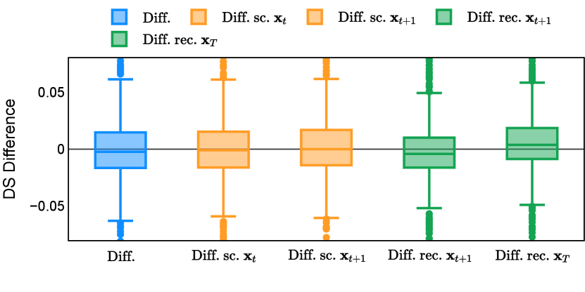
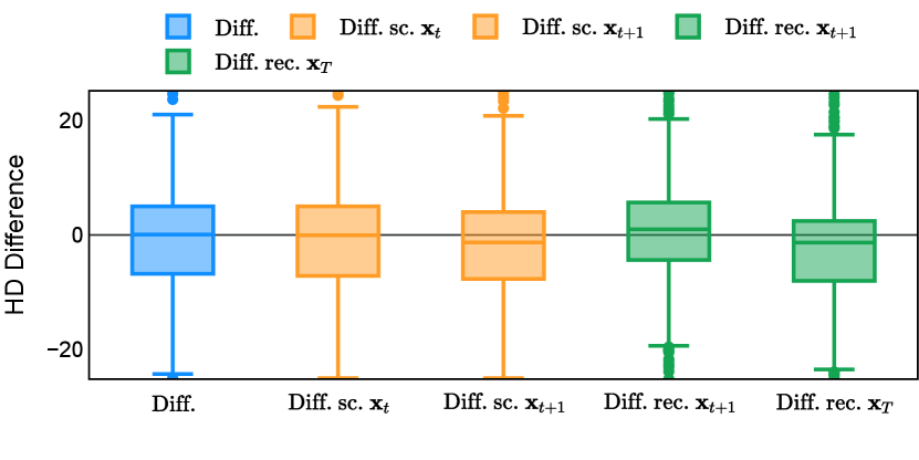
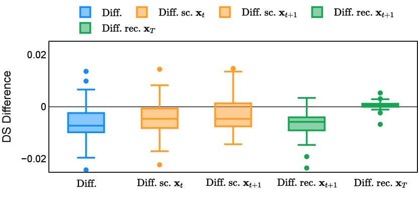
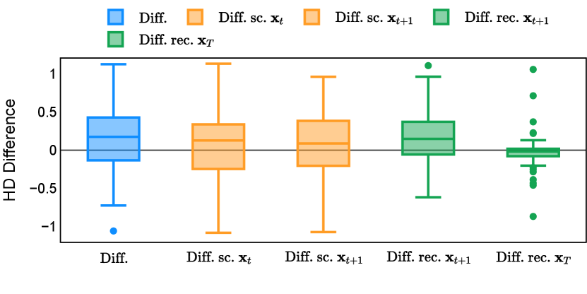
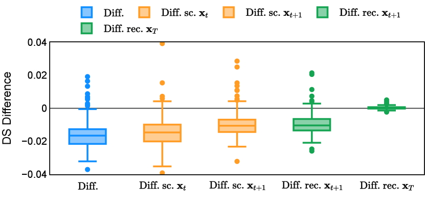
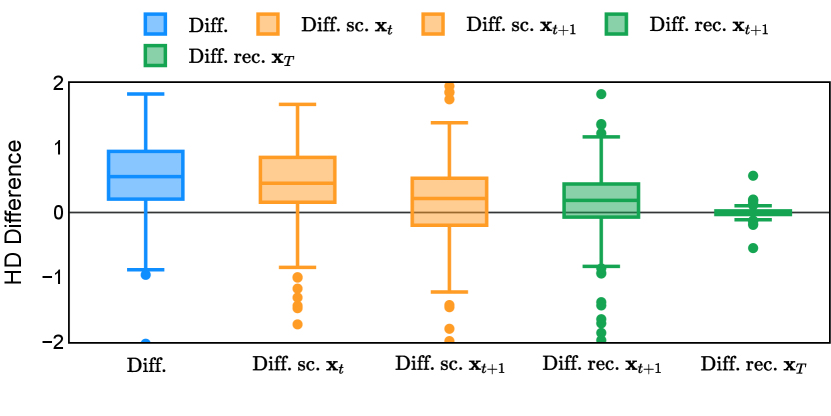
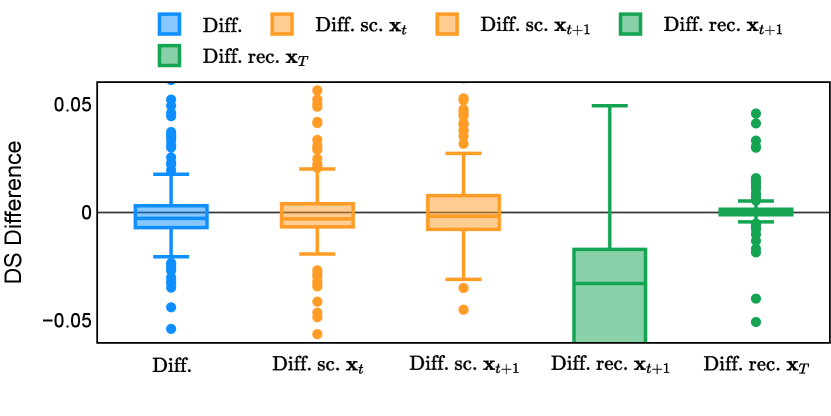
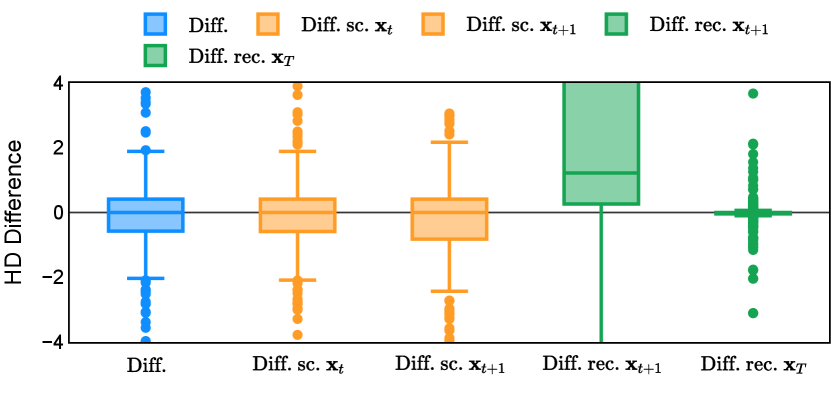
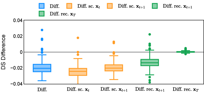
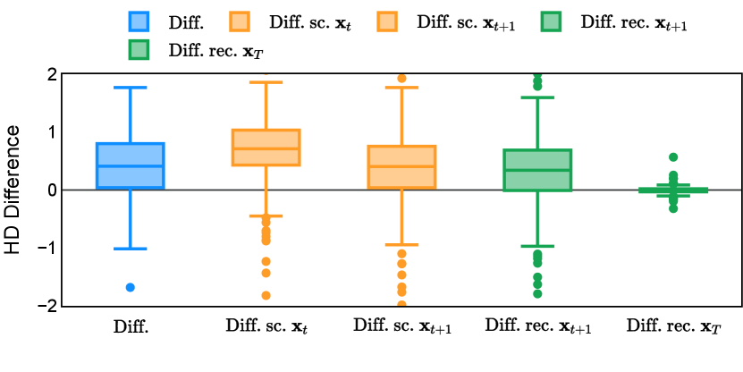
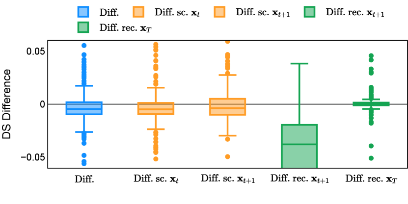
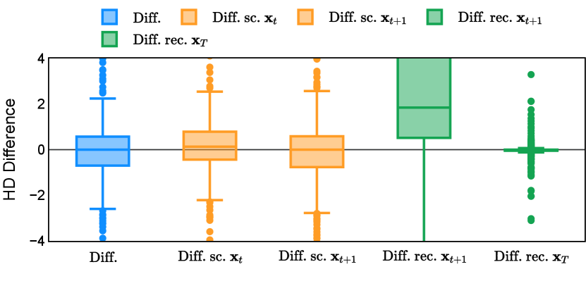
Different from deterministic models, the inference process of the diffusion model inherently incorporates stochasticity and models a distribution of the segmentation masks. Using the DDPM sampler with the proposed recycling-based diffusion model, the inference on each data set has been repeated with five different random seeds. Consequently, each sample has five distinct predicted masks. The maximum differences across five predictions were computed for the Dice score and Hausdorff distance, denoted by $\Delta$ Dice score and $\Delta$ Hausdorff distance, respectively. The average of this performance difference across all samples in the test set has been reported in Table 4 for all data sets. While the magnitude of the average difference (mean $\Delta$) varies across data sets, a common trend was observed where mean $\Delta$ diminished during the sampling process for both metrics. In other words, despite different initial predictions, the model’s predictions gradually converge as the difference across seeds decreases. Moreover, the relative magnitude of the mean $\Delta$ Hausdorff distance (e.g. $1.82$ at the last step for muscle ultrasound represents around $5\%$ fluctuation compared to $35.37$, the mean Hausdorff distance to ground truth) was larger than the relative magnitude for Dice score (e.g. $0.0051$ at the last step for muscle ultrasound was around $0.006\%$ fluctuation compared to $88.23$ the mean Hausdorff distance to ground truth). We hypothesize that the variation among predictions may predominantly revolve around local refinements in mask boundaries, as opposed to significant alterations like expansion or contraction of foreground areas. This may open a direction for further improving diffusion training: instead of performing independent noising per pixel/voxel results in fragmented and disjointed masks, the noising can be morphology-informed such that the noise-corrupted masks expand or contract the foreground with continuous boundaries.

6.3.3 Transformer

Table 5: Segmentation performance without Transformer. “No diff.” represents non-diffusion model. “Diff. rec. $\operatorname{\mathbf{x}}_{T}$” represents the diffusion model with proposed recycling. The inference sampler is DDPM. The best results are in bold and underline indicates the difference to non-diffusion model is significant with p-value < $0.05$.

Data Set	Method	Transformer	DS $\uparrow$	HD $\downarrow$
Muscle US	No diff.		86.66 $\pm$ 13.16	45.01 $\pm$ 38.86
		✓	88.15 $\pm$ 10.77	36.86 $\pm$ 30.04
	Diff. rec. $\operatorname{\mathbf{x}}_{T}$		88.36 $\pm$ 12.60	35.67 $\pm$ 34.12
		✓	88.23 $\pm$ 11.69	35.37 $\pm$ 31.79
Abdominal CT	No diff.		87.48 $\pm$ 5.02	6.63 $\pm$ 4.03
		✓	87.59 $\pm$ 5.10	6.36 $\pm$ 3.86
	Diff. rec. $\operatorname{\mathbf{x}}_{T}$		86.89 $\pm$ 5.49	6.91 $\pm$ 4.35
		✓	87.45 $\pm$ 5.43	6.56 $\pm$ 5.44
Prostate MR	No diff.		84.82 $\pm$ 5.69	4.55 $\pm$ 2.17
		✓	85.22 $\pm$ 5.18	4.62 $\pm$ 2.37
	Diff. rec. $\operatorname{\mathbf{x}}_{T}$		85.63 $\pm$ 5.19	4.59 $\pm$ 2.71
		✓	85.54 $\pm$ 5.20	4.40 $\pm$ 1.96
Brain MR	No diff.		92.03 $\pm$ 9.67	5.29 $\pm$ 8.53
		✓	92.43 $\pm$ 9.10	5.20 $\pm$ 9.56
	Diff. rec. $\operatorname{\mathbf{x}}_{T}$		92.04 $\pm$ 9.47	7.25 $\pm$ 13.76
		✓	92.29 $\pm$ 8.55	7.03 $\pm$ 13.48

Compared to Fu et al. (2023), the model includes a Transformer layer at the bottom encoder of U-net. This component has one layer representing 16% and 6% of the trainable parameters for 2D and 3D networks, correspondingly (see Table 7 in Section E). An ablation study has been performed for the proposed recycling approach and non-diffusion models. The results have been summarised in Table 5. For non-diffusion models, the addition of the Transformer component brought improvement in Dice score across all applications ($p<0.001$ for muscle ultrasound; $p>=0.05$ for abdominal CT; $p=0.001$ for prostate MR; and $p=0.0178$ for brain MR), making this architecture the stronger reference model. For diffusion, significantly higher Dice scores have been observed for abdominal CT data ($p<0.001$), and the differences were not significant for other applications ($p>=0.05$).

6.3.4 Length of training noise schedule

It’s worth noting that Fu et al. (2023) recommended incorporating a shortened variance schedule during training, mirroring that used during inference, in addition to the recycling technique. This modification resulted in enhanced performance for every training strategy on the muscle ultrasound data set (as detailed in LABEL:tab:timesteps_ablation_muscle). However, this adaptation did not yield enhancements for the proposed training strategies (“Diff. rec. $\operatorname{\mathbf{x}}_{T}$”) in the abdominal CT data set (as depicted in LABEL:tab:timesteps_ablation_abdominal). Moreover, not all differences observed were statistically significant. This may suggest that the advantage of the modified training variance schedule may be application-dependent and sensitive to the change of model architectures and hyper-parameters. In this work, the variance schedule was maintained at $1001$ steps.

7 Conclusion

In this research, we have proposed a novel training strategy for diffusion-based segmentation models. The aim is to remove the dependency on ground truth masks during denoising training. In contrast to the standard diffusion-based segmentation models and those employing self-conditioning or alternative recycling techniques, our approach consistently maintains or enhances segmentation performance throughout progressive inference processes. Through extensive experiments across four medical imaging data sets with different dimensionalities and modalities, we demonstrated statistically significant improvement against all diffusion baseline models for both DDPM and DDIM samplers. Our analysis for the first time identified a common limitation of existing diffusion model training for segmentation tasks. The use of ground truth data for denoising training leads to data leakage. By utilizing the model’s prediction at the initial step instead, we align the training process with inference procedures, effectively reducing over-fitting and promoting better generalization. While existing diffusion models underperformed non-diffusion-based segmentation model baselines, our innovative recycling training strategies effectively bridged the performance gap. This enhancement allowed diffusion models to attain comparable performance levels. To the best of our knowledge, this is the first time diffusion models have achieved such parity in performance while maintaining identical architecture and compute budget. By ensembling the diffusion and non-diffusion models, constant and significant improvements have been observed across all data sets, demonstrating one of its potential values. Nevertheless, challenges remain on the road to advancing diffusion-based segmentation models further. Future work could explore discrete diffusion models that are tailored for categorical data or implement diffusion in latent space to further reduce compute costs. Although the presented experimental results primarily demonstrated methodological development, the fact that these were obtained on four large clinical data sets represents a promising step toward real-world applications. We would like to argue the potential importance of the reported development, which may lead to better clinical outcomes and improved patient care in respective applications. For example, avoiding surrounding healthy structures may be sensitive to their localization in planning imaging, in both the abdominal CT and prostate MR tasks. This sensitivity can be high and nonlinear therefore arguably a perceived marginal improvement might benefit those with smaller targets, such as those in liver resection and focal therapy of prostate cancer, or highly variable ultrasound imaging guidance.

Acknowledgments

This work was supported by the EPSRC grant (EP/T029404/1), the Wellcome/EPSRC Centre for Interventional and Surgical Sciences (203145Z/16/Z), the International Alliance for Cancer Early Detection, an alliance between Cancer Research UK (C28070/A30912, C73666/A31378), Canary Center at Stanford University, the University of Cambridge, OHSU Knight Cancer Institute, University College London and the University of Manchester, and Cloud TPUs from Google’s TPU Research Cloud (TRC).

Ethical Standards

The work follows appropriate ethical standards in conducting research and writing the manuscript, following all applicable laws and regulations regarding treatment of animals or human subjects.

Conflicts of Interest

We declare we do not have conflicts of interest.

A Denoising Diffusion Probabilistic Model

We review the formulation of denoising diffusion probabilistic models (DDPM) from Sohl-Dickstein et al. (2015); Ho et al. (2020); Nichol and Dhariwal (2021).

A.1 Definition

$$\operatorname{\mathbf{x}}_{T}\autorightleftharpoons{}{}\cdots\autorightleftharpoons{}{}\operatorname{\mathbf{x}}_{t}\autorightleftharpoons{$p_{\theta}(\operatorname{\mathbf{x}}_{t-1}\mid\operatorname{\mathbf{x}}_{t})$}{$q(\operatorname{\mathbf{x}}_{t}\mid\operatorname{\mathbf{x}}_{t-1})$}\operatorname{\mathbf{x}}_{t-1}\autorightleftharpoons{}{}\cdots\autorightleftharpoons{}{}\operatorname{\mathbf{x}}_{0}$$

Consider a continuous diffusion process (also named forward process or noising process): given a data point $\operatorname{\mathbf{x}}_{0}\sim q(\operatorname{\mathbf{x}}_{0})$ in $\operatorname{\mathbb{R}}^{D}$, we add noise to $\operatorname{\mathbf{x}}_{t}$ for $t=1,\cdots,T$ with the following multivariate normal distribution:

$$q(\operatorname{\mathbf{x}}_{t}\mid\operatorname{\mathbf{x}}_{t-1})=\mathcal{N}(\operatorname{\mathbf{x}}_{t};\sqrt{1-\beta_{t}}\operatorname{\mathbf{x}}_{t-1},\beta_{t}\mathbf{I})$$

where $\beta_{t}\in[0,1]$ is a variance schedule. Given sufficiently large $T$ and a well-defined variance schedule, the distribution of $\operatorname{\mathbf{x}}_{T}$ approximates an isotropic multivariate normal distribution.

$$q(\operatorname{\mathbf{x}}_{t}\mid\operatorname{\mathbf{x}}_{0})\rightarrow\mathcal{N}(\operatorname{\mathbf{x}}_{t};\mathbf{0},\mathbf{I})$$

Therefore, we can define a reverse process (also named denoising process): given a sample $\operatorname{\mathbf{x}}_{T}\sim\mathcal{N}(\operatorname{\mathbf{x}}_{T};\mathbf{0},\mathbf{I})$, we denoise the data using neural networks $\bm{\mu}_{\theta}:\operatorname{\mathbb{R}}^{D}\rightarrow\operatorname{\mathbb{R}}^{D}$ and $\mathbf{\Sigma}_{\theta}:\operatorname{\mathbb{R}}^{D}\rightarrow\operatorname{\mathbb{R}}^{D\times D}$ as follows:

$$p_{\theta}(\operatorname{\mathbf{x}}_{t-1}\mid\operatorname{\mathbf{x}}_{t})=\mathcal{N}(\operatorname{\mathbf{x}}_{t-1};\bm{\mu}_{\theta}(\operatorname{\mathbf{x}}_{t},t),\mathbf{\Sigma}_{\theta}(\operatorname{\mathbf{x}}_{t},t))$$

In this work, an isotropic variance is assumed with $\mathbf{\Sigma}_{\theta}(\operatorname{\mathbf{x}}_{t},t)=\sigma_{t}^{2}\mathbf{I}$, such that

$$p_{\theta}(\operatorname{\mathbf{x}}_{t-1}\mid\operatorname{\mathbf{x}}_{t})=\mathcal{N}(\operatorname{\mathbf{x}}_{t-1};\bm{\mu}_{\theta}(\operatorname{\mathbf{x}}_{t},t),\sigma_{t}^{2}\mathbf{I})$$

A.2 Variational Lower Bound

Consider $\operatorname{\mathbf{z}}=\operatorname{\mathbf{x}}_{1:T}\mid\operatorname{\mathbf{x}}_{0}$ as latent variables for $\operatorname{\mathbf{x}}_{0}$, we can derive the variational lower bound (VLB) as follows:

$$\log p_{\theta}(\operatorname{\mathbf{x}}_{0})= D_{\text{KL}}(q(\operatorname{\mathbf{z}})\leavevmode\nobreak\ \|\leavevmode\nobreak\ p_{\theta}(\operatorname{\mathbf{z}}\mid\operatorname{\mathbf{x}}_{0}))+\operatorname{\mathbb{E}}_{q(\operatorname{\mathbf{z}})}\left[\log\frac{p_{\theta}(\operatorname{\mathbf{x}}_{0},\operatorname{\mathbf{z}})}{q(\operatorname{\mathbf{z}})}\right]$$

$$\geq \operatorname{\mathbb{E}}_{q(\operatorname{\mathbf{z}})}\left[\log\frac{p_{\theta}(\operatorname{\mathbf{x}}_{0},\operatorname{\mathbf{z}})}{q(\operatorname{\mathbf{z}})}\right]$$

$$= -\Big{(}\operatorname{\mathbb{E}}_{q(\operatorname{\mathbf{x}}_{1}\mid\operatorname{\mathbf{x}}_{0})}L_{0}+\sum_{t=2}^{T}\operatorname{\mathbb{E}}_{q(\operatorname{\mathbf{x}}_{t}\mid\operatorname{\mathbf{x}}_{0})}L_{t-1}+L_{T}\Big{)}$$

where

$$L_{0} =-\log p_{\theta}(\operatorname{\mathbf{x}}_{0}\mid\operatorname{\mathbf{x}}_{1})$$(reconstruction loss)

$$L_{t-1} =D_{\text{KL}}(q(\operatorname{\mathbf{x}}_{t-1}\mid\operatorname{\mathbf{x}}_{t},\operatorname{\mathbf{x}}_{0})\|p_{\theta}(\operatorname{\mathbf{x}}_{t-1}\mid\operatorname{\mathbf{x}}_{t}))$$(diffussion loss)

$$L_{T} =D_{\text{KL}}(q(\operatorname{\mathbf{x}}_{T}\mid\operatorname{\mathbf{x}}_{0}))\leavevmode\nobreak\ \|\leavevmode\nobreak\ p_{\theta}(\operatorname{\mathbf{x}}_{T}).$$(prior loss)

A.3 Diffusion Loss

In particular, we can derive the closed form $L_{t-1}$ with

$$q(\operatorname{\mathbf{x}}_{t}\mid\operatorname{\mathbf{x}}_{0}) =\mathcal{N}(\operatorname{\mathbf{x}}_{t};\sqrt{\bar{\alpha}_{t}}\operatorname{\mathbf{x}}_{0},(1-\bar{\alpha}_{t})\mathbf{I})$$

$$q(\operatorname{\mathbf{x}}_{t-1}\mid\operatorname{\mathbf{x}}_{t},\operatorname{\mathbf{x}}_{0}) =\mathcal{N}(\operatorname{\mathbf{x}}_{t-1};\tilde{\bm{\mu}}(\operatorname{\mathbf{x}}_{t},\operatorname{\mathbf{x}}_{0}),\tilde{\beta}_{t}\mathbf{I})$$

where

$$\alpha_{t} =1-\beta_{t}$$

$$\bar{\alpha}_{t} =\prod_{s=1}^{t}\alpha_{s}$$

$$\tilde{\bm{\mu}}(\operatorname{\mathbf{x}}_{t},\operatorname{\mathbf{x}}_{0}) =\frac{\sqrt{\bar{\alpha}_{t-1}}\beta_{t}}{1-\bar{\alpha}_{t}}\operatorname{\mathbf{x}}_{0}+\frac{1-\bar{\alpha}_{t-1}}{1-\bar{\alpha}_{t}}\sqrt{\alpha_{t}}\operatorname{\mathbf{x}}_{t},$$(88)

$$\tilde{\beta}_{t} =\frac{1-\bar{\alpha}_{t-1}}{1-\bar{\alpha}_{t}}\beta_{t}.$$

A.3.1 Noise Prediction Loss ($\epsilon$-parameterization)s

Consider the reparameterization in Ho et al. (2020),

$$\operatorname{\mathbf{x}}_{t}(\operatorname{\mathbf{x}}_{0},\operatorname{\bm{\epsilon}}) =\sqrt{\bar{\alpha}_{t}}\operatorname{\mathbf{x}}_{0}+\sqrt{1-\bar{\alpha}_{t}}\operatorname{\bm{\epsilon}}$$

$$\operatorname{\bm{\epsilon}}_{\theta}(\operatorname{\mathbf{x}}_{t},t) =\frac{1}{\sqrt{1-\bar{\alpha}_{t}}}\operatorname{\mathbf{x}}_{t}-\frac{\sqrt{\bar{\alpha}_{t}}}{\sqrt{1-\bar{\alpha}_{t}}}\operatorname{\mathbf{x}}_{0}$$

$$\bm{\mu}_{\theta}(\operatorname{\mathbf{x}}_{t},t) =\frac{1}{\sqrt{\alpha}_{t}}(\operatorname{\mathbf{x}}_{t}-\frac{\beta_{t}}{\sqrt{1-\bar{\alpha}_{t}}}\operatorname{\bm{\epsilon}}_{\theta}(\operatorname{\mathbf{x}}_{t},t))$$

We can derive a closed form of $L_{t-1}$

$$L_{t-1}(\operatorname{\mathbf{x}}_{t},\operatorname{\mathbf{x}}_{0})=\frac{1}{2\sigma_{t}^{2}}\frac{\beta_{t}^{2}}{{\alpha_{t}(1-\bar{\alpha}_{t})}}\|\operatorname{\bm{\epsilon}}-\operatorname{\bm{\epsilon}}_{\theta}\|_{2}^{2}+C$$

If $\sigma_{t}^{2}=\tilde{\beta}_{t}=\frac{1-\bar{\alpha}_{t-1}}{1-\bar{\alpha}_{t}}\beta_{t}$, using the signal-to-noise ratio (SNR) defined in  Kingma et al. (2021), $\text{SNR}(t)=\frac{\bar{\alpha}_{t}}{1-\bar{\alpha}_{t}}$, the loss can be derived as

$$L_{t-1}(\operatorname{\mathbf{x}}_{t},\operatorname{\mathbf{x}}_{0})=(\frac{\text{SNR}(t-1)}{\text{SNR}(t)}-1)\|\operatorname{\bm{\epsilon}}-\operatorname{\bm{\epsilon}}_{\theta}\|_{2}^{2}+C$$

A.3.2 Sample Prediction Loss ($\operatorname{\mathbf{x}}_{0}$-parameterization)

Similar to Eq. 88, consider the parameterization (Kingma et al., 2021),

$$\bm{\mu}_{\theta}(\operatorname{\mathbf{x}}_{t},t)=\frac{\sqrt{\bar{\alpha}_{t-1}}\beta_{t}}{1-\bar{\alpha}_{t}}\operatorname{\mathbf{x}}_{0,\theta}+\frac{1-\bar{\alpha}_{t-1}}{1-\bar{\alpha}_{t}}\sqrt{\alpha_{t}}\operatorname{\mathbf{x}}_{t}$$

We can derive a closed form of $L_{t-1}$

$$L_{t-1}(\operatorname{\mathbf{x}}_{t},\operatorname{\mathbf{x}}_{0})=\frac{1}{2\sigma_{t}^{2}}\frac{\bar{\alpha}_{t-1}\beta_{t}^{2}}{(1-\bar{\alpha}_{t})^{2}}\|\operatorname{\mathbf{x}}_{0,\theta}-\operatorname{\mathbf{x}}_{0}\|_{2}^{2}+C.$$

If $\sigma_{t}^{2}=\tilde{\beta}_{t}=\frac{1-\bar{\alpha}_{t-1}}{1-\bar{\alpha}_{t}}\beta_{t}$, using the signal-to-noise ratio (SNR) defined in  Kingma et al. (2021), $\text{SNR}(t)=\frac{\bar{\alpha}_{t}}{1-\bar{\alpha}_{t}}$, the loss can be derived as

$$L_{t-1}(\operatorname{\mathbf{x}}_{t},\operatorname{\mathbf{x}}_{0})=\frac{1}{2}(\text{SNR}(t-1)-\text{SNR}(t))\|\operatorname{\mathbf{x}}_{0,\theta}-\operatorname{\mathbf{x}}_{0}\|_{2}^{2}+C.$$

A.4 Training

Empirically, instead of using the variational lower bound, the neural network can be trained on one of the following simplified loss (Ho et al., 2020)

$$L_{\text{simple},\operatorname{\bm{\epsilon}}_{t}}(\theta) =\operatorname{\mathbb{E}}_{t,\operatorname{\mathbf{x}}_{0},\operatorname{\bm{\epsilon}}_{t}}\|\operatorname{\bm{\epsilon}}_{t}-\operatorname{\bm{\epsilon}}_{t,\theta}\|_{2}^{2}=\operatorname{\mathbb{E}}_{t,\operatorname{\mathbf{x}}_{0},\operatorname{\bm{\epsilon}}_{t}}L(\operatorname{\bm{\epsilon}}_{t},\operatorname{\bm{\epsilon}}_{t,\theta}),\leavevmode\nobreak\ (\operatorname{\bm{\epsilon}}\text{-parameterization})$$

$$L_{\text{simple},\operatorname{\mathbf{x}}_{0}}(\theta) =\operatorname{\mathbb{E}}_{t,\operatorname{\mathbf{x}}_{0},\operatorname{\bm{\epsilon}}_{t}}\|\operatorname{\mathbf{x}}_{0}-\operatorname{\mathbf{x}}_{0,\theta}\|_{2}^{2}=\operatorname{\mathbb{E}}_{t,\operatorname{\mathbf{x}}_{0},\operatorname{\bm{\epsilon}}_{t}}L(\operatorname{\mathbf{x}}_{0},\operatorname{\mathbf{x}}_{0,\theta}).\leavevmode\nobreak\ (\operatorname{\mathbf{x}}_{0}\text{-parameterization})$$

with $t$ uniformly sampled from $1$ to $T$ and $\operatorname{\bm{\epsilon}}_{t}\sim\mathcal{N}(\mathbf{0},\mathbf{I})$. $L(\cdot,\cdot)$ is a loss function in the space of $\operatorname{\mathbf{x}}$. With the importance sampling proposed in Nichol and Dhariwal (2021), $t$ can be sampled with a probability proportional to $\operatorname{\mathbb{E}}_{\operatorname{\mathbf{x}}_{0},\operatorname{\mathbf{x}}_{t}}L(\operatorname{\mathbf{x}}_{0},\hat{\operatorname{\mathbf{x}}}_{0})$. In other words, a time step $t$ is sampled more often if the loss is larger.

As the previous work (Fu et al., 2023) has extensively compared the $\operatorname{\bm{\epsilon}}$-parameterization and $\operatorname{\mathbf{x}}_{0}$-parameterization, as well as the benefits of including Dice loss, in this work, we use $\operatorname{\mathbf{x}}_{0}$-parameterization with a weighted sum of cross-entropy and foreground-only Dice loss Kirillov et al. (2023).

A.5 Variance Resampling

Given a variance schedule $\{\beta_{t}\}_{t=1}^{T}$ (e.g. $T=1001$), a subsequence $\{\beta_{k}\}_{k=1}^{K}$ (e.g. $K=5$) can be sampled with $\{t_{k}\}_{k=1}^{K}$. Following Nichol and Dhariwal (2021), we can define $\beta_{k}=1-\frac{\bar{\alpha}_{t_{k}}}{\bar{\alpha}_{t_{k-1}}}$ then $\alpha_{k}=1-\beta_{k}$ and $\bar{\alpha}_{k}=\prod_{s=1}^{k}\alpha_{s}$ can be recalculated correspondingly. In this work, $t_{k}$ is uniformly downsampled. For instance, if $T=1001$ and $K=5$, then $\{t_{k}\}_{k=1}^{K}=\{1,251,501,751,1001\}$.

B Denoising Diffusion Implicit Model

Definition

Song et al. (2020a) parameterize $q(\operatorname{\mathbf{x}}_{t-1}\mid\operatorname{\mathbf{x}}_{t},\operatorname{\mathbf{x}}_{0})$ as follows, with $\operatorname{\bm{\epsilon}}=\frac{\operatorname{\mathbf{x}}_{t}-\sqrt{\bar{\alpha}_{t}}\operatorname{\mathbf{x}}_{0}}{\sqrt{1-\bar{\alpha}_{t}}}$,

$$q(\operatorname{\mathbf{x}}_{t-1}\mid\operatorname{\mathbf{x}}_{t},\operatorname{\mathbf{x}}_{0}) =\mathcal{N}(\operatorname{\mathbf{x}}_{t-1};\sqrt{\bar{\alpha}_{t-1}}\operatorname{\mathbf{x}}_{0}+\sqrt{1-\bar{\alpha}_{t-1}-\sigma_{t}}\operatorname{\bm{\epsilon}},\sigma_{t}^{2}\mathbf{I}).$$

For any variance schedule $\sigma_{t}$, this formulation ensures $q(\operatorname{\mathbf{x}}_{t}\mid\operatorname{\mathbf{x}}_{0})=\mathcal{N}(\operatorname{\mathbf{x}}_{t};\sqrt{\bar{\alpha}_{t}}\operatorname{\mathbf{x}}_{0},(1-\bar{\alpha}_{t})\mathbf{I})$. Particularly, if $\sigma_{t}^{2}=\tilde{\beta}_{t}$, this represents DDPM. If $\sigma_{t}=0$ for $t>1$ and $\sigma_{1}=\sqrt{\tilde{\beta}_{1}}$, the model is deterministic and named as denoising diffusion implicit model (DDIM).

Inference

For DDIM, at inference time, the denoising starts with a Gaussian noise $\operatorname{\mathbf{x}}_{T}\sim\mathcal{N}(\bm{0},\bm{I})$ and the data is denoised step-by-step for $t=T,\cdots,1$:

$$p_{\theta}(\operatorname{\mathbf{x}}_{t-1}\mid\operatorname{\mathbf{x}}_{t})=\begin{cases}\mathcal{N}(\hat{\operatorname{\mathbf{x}}}_{0},\sigma_{1}^{2}\mathbf{I})&t=1\\ q(\operatorname{\mathbf{x}}_{t-1}\mid\operatorname{\mathbf{x}}_{t},\operatorname{\mathbf{x}}_{0,\theta}(\operatorname{\mathbf{x}}_{t},t))&t>1\end{cases}$$

C Self-conditioning

The self-conditioning methods proposed in Chen et al. (2022b) (“Diff. sc. $\operatorname{\mathbf{x}}_{t}$” in Equation 89) and Watson et al. (2023) (“sc. $\operatorname{\mathbf{x}}_{t+1}$” in Equation 90) are illustrated below.

$$\operatorname{\mathbf{x}}_{t} \sim\mathcal{N}(\operatorname{\mathbf{x}}_{t};\sqrt{\bar{\alpha}_{t}}\mathbf{x}_{0},(1-\bar{\alpha}_{t})\mathbf{I}), (\text{sc.}\leavevmode\nobreak\ \operatorname{\mathbf{x}}_{t},\leavevmode\nobreak\ \text{step 1, sampling})$$(89a)

$$\hat{\mathbf{x}}_{0} =\text{StopGradient}(f_{\theta}(I,t,\mathbf{x}_{t},\mathbf{0})), (\text{sc.}\leavevmode\nobreak\ \operatorname{\mathbf{x}}_{t},\leavevmode\nobreak\ \text{step 1, prediction})$$(89b)

$$\hat{\mathbf{x}}_{0} =\text{Dropout}_{p=50\%}(\hat{\mathbf{x}}_{0}), (\text{sc.}\leavevmode\nobreak\ \operatorname{\mathbf{x}}_{t},\leavevmode\nobreak\ \text{step 2, dropout})$$(89c)

$$\hat{\mathbf{x}}_{0} =f_{\theta}(I,t,\mathbf{x}_{t},\hat{\mathbf{x}}_{0}), (\text{sc.}\leavevmode\nobreak\ \operatorname{\mathbf{x}}_{t},\leavevmode\nobreak\ \text{step 2, prediction})$$(89d)

$$L_{\text{denoising}}(\theta) =\operatorname{\mathbb{E}}_{t,\operatorname{\mathbf{x}}_{0},\operatorname{\mathbf{x}}_{t}}L(\operatorname{\mathbf{x}}_{0},\hat{\mathbf{x}}_{0}), (\text{loss calculation})$$(89e)

$$\operatorname{\mathbf{x}}_{t+1} \sim\mathcal{N}(\operatorname{\mathbf{x}}_{t+1};\sqrt{\bar{\alpha}_{t+1}}\operatorname{\mathbf{x}}_{0},(1-\bar{\alpha}_{t+1})\mathbf{I}), (\text{sc.}\leavevmode\nobreak\ \operatorname{\mathbf{x}}_{t+1},\leavevmode\nobreak\ \text{step 1, sampling})$$(90a)

$$\hat{\mathbf{x}}_{0} =\text{StopGradient}(f_{\theta}(I,t+1,\mathbf{x}_{t+1},\mathbf{0})), (\text{sc.}\leavevmode\nobreak\ \operatorname{\mathbf{x}}_{t+1},\leavevmode\nobreak\ \text{step 1, prediction})$$(90b)

$$\hat{\mathbf{x}}_{0} =\text{Dropout}_{p=50\%}(\hat{\mathbf{x}}_{0}), (\text{sc.}\leavevmode\nobreak\ \operatorname{\mathbf{x}}_{t+1},\leavevmode\nobreak\ \text{step 2, dropout})$$(90c)

$$\operatorname{\mathbf{x}}_{t} \sim\mathcal{N}(\operatorname{\mathbf{x}}_{t};\tilde{\bm{\mu}},\tilde{\beta}_{t+1}\mathbf{I}), (\text{sc.}\leavevmode\nobreak\ \operatorname{\mathbf{x}}_{t+1},\leavevmode\nobreak\ \text{step 2, sampling})$$(90d)

$$\tilde{\bm{\mu}} =\frac{\sqrt{\bar{\alpha}_{t}}\beta_{t+1}}{1-\bar{\alpha}_{t+1}}\operatorname{\mathbf{x}}_{0}+\frac{1-\bar{\alpha}_{t}}{1-\bar{\alpha}_{t+1}}\sqrt{\alpha_{t+1}}\operatorname{\mathbf{x}}_{t+1}$$

$$\hat{\mathbf{x}}_{0} =f_{\theta}(I,t,\mathbf{x}_{t},\hat{\mathbf{x}}_{0}), (\text{sc.}\leavevmode\nobreak\ \operatorname{\mathbf{x}}_{t+1},\leavevmode\nobreak\ \text{step 2, prediction})$$(90e)

$$L_{\text{denoising}}(\theta) =\operatorname{\mathbb{E}}_{t,\operatorname{\mathbf{x}}_{0},\operatorname{\mathbf{x}}_{t}}L(\operatorname{\mathbf{x}}_{0},\hat{\mathbf{x}}_{0}), (\text{loss calculation})$$(90f)

D Diffusion Noise Schedule

The noise schedule $\beta_{t}$ and $\sqrt{\bar{\alpha}_{t}}$ have been visualised in Figure 2. The cross entropy and dice score between $\operatorname{\mathbf{x}}_{t}$ and ground truth $\operatorname{\mathbf{x}}_{0}$ have also been visualized to empirically measure the amount of information of ground truth $\operatorname{\mathbf{x}}_{0}$ contained in $\operatorname{\mathbf{x}}_{t}$.

(a) $\beta_{t}$

(b) $\sqrt{\bar{\alpha_{t}}}$

(c) Cross entropy

(d) Dice score

Figure 2: Information contained in $\operatorname{\mathbf{x}}_{t}$. Cross entropy and dice score between $\operatorname{\mathbf{x}}_{t}$ and ground truth $\operatorname{\mathbf{x}}_{0}$ are used to empirically measure the amount of information of ground truth $\operatorname{\mathbf{x}}_{0}$ contained in $\operatorname{\mathbf{x}}_{t}$. The dashed line represents the information contained in the sampled noise (between noise and ground truth $\operatorname{\mathbf{x}}_{0}$), which is considered to be the limit. The values are calculated using the sample “005095” in prostate MR data set.

E Implementation Details

Table 6: Training Hyper-parameters

Parameter	Value
Optimiser	AdamW (b1=0.9, b2=0.999, weight_decay=1E-8)
Learning Rate Warmup	100 steps
Learning Rate Decay	10,000 steps
Learning Rate Values	Initial = 1E-5, Peak = 8E-4, End = 5E-5
Batch size	256 for Muscle Ultrasound and 8 for other data sets
Number of samples	320K for Muscle Ultrasound and 100K for other data sets

Table 7: Network Size

Dimension	Method	Transformer
		✓
2D	No diff.	12,586,594	10,550,370
	Diff.	13,335,554	11,299,330
3D	No diff.	33,385,154	31,283,394
	Diff.	34,135,266	32,033,506

F Results

F.1 Diffusion Training Strategy Comparison

Table 8: Per class Dice score comparison. “No diff.” represents non-diffusion model. “Diff. rec. $\operatorname{\mathbf{x}}_{T}$” represents the diffusion model with proposed recycling. “Ensemble” represents the model averaging the probabilities from “No diff.” and “Diff. rec. $\operatorname{\mathbf{x}}_{T}$”. The inference sampler is DDPM. The best results are in bold and underline indicates the difference to non-diffusion model is significant with p-value < $0.05$.

Method	Spleen	RT kidney	LT kidney	Gall bladder
No diff.	96.62 $\pm$ 1.87	95.08 $\pm$ 10.74	96.29 $\pm$ 1.73	78.83 $\pm$ 27.82
Diff. rec. $\operatorname{\mathbf{x}}_{T}$	96.40 $\pm$ 2.42	96.24 $\pm$ 1.90	96.27 $\pm$ 1.53	76.68 $\pm$ 29.25
Ensemble	96.78 $\pm$ 1.75	96.47 $\pm$ 2.44	96.50 $\pm$ 1.51	79.65 $\pm$ 27.29
Method	Esophagus	Liver	Stomach	Arota
No diff.	83.22 $\pm$ 11.08	97.36 $\pm$ 1.17	90.53 $\pm$ 14.78	94.65 $\pm$ 4.22
Diff. rec. $\operatorname{\mathbf{x}}_{T}$	83.60 $\pm$ 10.32	97.33 $\pm$ 1.13	90.77 $\pm$ 14.46	94.66 $\pm$ 4.66
Ensemble	84.10 $\pm$ 11.15	97.54 $\pm$ 1.05	91.07 $\pm$ 14.91	94.96 $\pm$ 4.39
Method	Postcava	Pancreas	Right adrenal gland	Left adrenal gland
No diff.	90.45 $\pm$ 4.68	84.88 $\pm$ 11.40	77.80 $\pm$ 9.46	77.98 $\pm$ 11.95
Diff. rec. $\operatorname{\mathbf{x}}_{T}$	90.55 $\pm$ 4.19	84.86 $\pm$ 11.15	76.63 $\pm$ 12.84	78.01 $\pm$ 11.60
Ensemble	91.18 $\pm$ 4.12	85.85 $\pm$ 11.12	78.51 $\pm$ 10.58	78.95 $\pm$ 11.45
Method	Duodenum	Bladder	Prostate/uterus
No diff.	79.57 $\pm$ 14.89	88.09 $\pm$ 16.25	82.35 $\pm$ 18.90
Diff. rec. $\operatorname{\mathbf{x}}_{T}$	79.80 $\pm$ 15.14	87.90 $\pm$ 16.65	81.90 $\pm$ 18.86
Ensemble	80.99 $\pm$ 15.07	88.61 $\pm$ 16.59	83.06 $\pm$ 18.68

(a) Abdominal CT: LT and RT stand for left and right, respectively.

Method	Bladder	Bone	Obturator internus	Transition zone
No diff.	93.28 $\pm$ 9.90	93.12 $\pm$ 5.68	88.95 $\pm$ 3.53	79.61 $\pm$ 8.37
Diff. rec. $\operatorname{\mathbf{x}}_{T}$	93.57 $\pm$ 9.61	93.84 $\pm$ 5.85	89.15 $\pm$ 3.62	79.79 $\pm$ 8.36
Ensemble	93.66 $\pm$ 9.84	93.77 $\pm$ 5.52	89.52 $\pm$ 3.51	80.57 $\pm$ 8.20
Method	Central gland	Rectum	Seminal vesicle	NV bundle
No diff.	88.75 $\pm$ 5.60	93.30 $\pm$ 3.48	77.55 $\pm$ 10.99	67.17 $\pm$ 14.34
Diff. rec. $\operatorname{\mathbf{x}}_{T}$	89.13 $\pm$ 5.78	93.42 $\pm$ 3.51	78.39 $\pm$ 9.71	67.07 $\pm$ 15.50
Ensemble	89.45 $\pm$ 5.56	93.70 $\pm$ 3.37	78.91 $\pm$ 10.28	68.01 $\pm$ 14.85

(b) Prostate MR: Dice score per class. NV stands for neurovascular.

Table 9: Per class Hausdorff distance comparison “No diff.” represents non-diffusion model. “Diff. rec. $\operatorname{\mathbf{x}}_{T}$” represents the diffusion model with proposed recycling. “Ensemble” represents the model averaging the probabilities from “No diff.” and “Diff. rec. $\operatorname{\mathbf{x}}_{T}$”. The inference sampler is DDPM. The best results are in bold and underline indicates the difference to non-diffusion model is significant with p-value < $0.05$.

Method	Spleen	Right kidney	Left kidney	Gall bladder
No diff.	3.22 $\pm$ 4.91	1.97 $\pm$ 1.46	4.13 $\pm$ 10.83	9.23 $\pm$ 16.71
Diff. rec. $\operatorname{\mathbf{x}}_{T}$	2.86 $\pm$ 3.84	1.93 $\pm$ 0.83	3.13 $\pm$ 8.35	12.65 $\pm$ 21.74
Ensemble	2.89 $\pm$ 4.28	1.84 $\pm$ 1.11	2.70 $\pm$ 5.86	9.57 $\pm$ 18.86
Method	Esophagus	Liver	Stomach	Arota
No diff.	5.50 $\pm$ 6.81	3.50 $\pm$ 2.50	8.96 $\pm$ 13.99	6.62 $\pm$ 14.52
Diff. rec. $\operatorname{\mathbf{x}}_{T}$	5.30 $\pm$ 6.41	3.79 $\pm$ 4.16	9.00 $\pm$ 14.03	5.41 $\pm$ 11.20
Ensemble	5.22 $\pm$ 6.63	3.06 $\pm$ 1.63	8.04 $\pm$ 12.87	5.47 $\pm$ 11.29
Method	Postcava	Pancreas	Right adrenal gland	Left adrenal gland
No diff.	4.80 $\pm$ 4.55	7.57 $\pm$ 8.62	4.39 $\pm$ 2.39	5.15 $\pm$ 5.40
Diff. rec. $\operatorname{\mathbf{x}}_{T}$	4.62 $\pm$ 3.09	7.50 $\pm$ 8.62	4.66 $\pm$ 3.14	4.87 $\pm$ 4.64
Ensemble	4.41 $\pm$ 3.25	6.96 $\pm$ 8.40	4.41 $\pm$ 2.79	4.82 $\pm$ 4.92
Method	Duodenum	Bladder	Prostate/uterus
No diff.	10.54 $\pm$ 8.44	9.10 $\pm$ 23.07	10.97 $\pm$ 19.01
Diff. rec. $\operatorname{\mathbf{x}}_{T}$	9.31 $\pm$ 7.13	10.70 $\pm$ 31.83	13.35 $\pm$ 32.75
Ensemble	9.29 $\pm$ 7.37	6.52 $\pm$ 10.34	9.14 $\pm$ 13.11

(a) Abdominal CT: LT and RT stand for left and right, respectively.

Method	Bladder	Bone	Obturator internus	Transition zone
No diff.	3.30 $\pm$ 4.54	3.18 $\pm$ 9.77	4.60 $\pm$ 3.36	5.97 $\pm$ 4.97
Diff. rec. $\operatorname{\mathbf{x}}_{T}$	3.20 $\pm$ 4.12	2.21 $\pm$ 1.62	4.50 $\pm$ 3.46	6.25 $\pm$ 4.96
Ensemble	2.95 $\pm$ 3.48	2.32 $\pm$ 1.46	4.34 $\pm$ 3.29	6.18 $\pm$ 5.11
Method	Central gland	Rectum	Seminal vesicle	NV bundle
No diff.	3.94 $\pm$ 2.28	4.46 $\pm$ 5.69	4.82 $\pm$ 3.85	6.68 $\pm$ 6.33
Diff. rec. $\operatorname{\mathbf{x}}_{T}$	3.70 $\pm$ 1.93	4.25 $\pm$ 4.75	4.57 $\pm$ 2.66	6.55 $\pm$ 6.28
Ensemble	3.66 $\pm$ 1.93	4.16 $\pm$ 5.25	4.52 $\pm$ 2.83	6.45 $\pm$ 6.34

(b) Prostate MR: Dice score per class. NV stands for neurovascular.

(a) DS difference for muscle ultrasound

(b) HD difference for muscle ultrasound

(c) DS difference for abdominal CT

(d) HD difference for abdominal CT

(e) DS difference for prostate MR

(f) HD difference for prostate MR

(g) DS difference for brain MR

(h) HD difference for brain MR

Figure 3: Segmentation performance difference between the last step and first step using DDPM. “Diff.” represents standard diffusion. “Diff. sc. $\operatorname{\mathbf{x}}_{t}$” and “Diff. sc. $\operatorname{\mathbf{x}}_{t+1}$” represents self-conditioning from Chen et al. (2022b) and Watson et al. (2023), respectively. “Diff. rec. $\operatorname{\mathbf{x}}_{t+1}$” and “Diff. rec. $\operatorname{\mathbf{x}}_{T}$” represents recycling from Fu et al. (2023) and the proposed recycling in this work, respectively. The sampler is DDPM. DS and HD represents Dice score and Hausdorff distance, respectively. The difference is the value at the last step subtracted by the one at the first step. A positive value for Dice score difference or a negative value for Hausdorff distance means improvement.

(a) DS difference for muscle ultrasound

(b) HD difference for muscle ultrasound

(c) DS difference for abdominal CT

(d) HD difference for abdominal CT

(e) DS difference for prostate MR

(f) HD difference for prostate MR

(g) DS difference for brain MR

(h) HD difference for brain MR

Figure 4: Segmentation performance difference between the last step and first step using DDIM. “Diff.” represents standard diffusion. “Diff. sc. $\operatorname{\mathbf{x}}_{t}$” and “Diff. sc. $\operatorname{\mathbf{x}}_{t+1}$” represents self-conditioning from Chen et al. (2022b) and Watson et al. (2023), respectively. “Diff. rec. $\operatorname{\mathbf{x}}_{t+1}$” and “Diff. rec. $\operatorname{\mathbf{x}}_{T}$” represents recycling from Fu et al. (2023) and the proposed recycling in this work, respectively. The sampler is DDIM. DS and HD represents Dice score and Hausdorff distance, respectively. The difference is the value at the last step subtracted by the one at the first step. A positive value for Dice score difference or a negative value for Hausdorff distance means improvement.

(a) Dice Score for muscle ultrasound

(b) Hausdorff distance for muscle ultrasound

(c) Dice score for abdominal CT

(d) Hausdorff distance for abdominal CT

(e) Dice score for prostate MR

(f) Hausdorff distance for prostate MR

(g) Dice score for brain MR

(h) Hausdorff distance for brain MR

Figure 5: Segmentation performance per step. “Diff.” represents standard diffusion. “Diff. sc. $\operatorname{\mathbf{x}}_{t}$” and “Diff. sc. $\operatorname{\mathbf{x}}_{t+1}$” represents self-conditioning from Chen et al. (2022b) and Watson et al. (2023), respectively. “Diff. rec. $\operatorname{\mathbf{x}}_{t+1}$” and “Diff. rec. $\operatorname{\mathbf{x}}_{T}$” represents recycling from Fu et al. (2023) and the proposed recycling in this work, respectively. The sampler is DDIM.

References

- Amit et al. (2021) Tomer Amit, Eliya Nachmani, Tal Shaharbany, and Lior Wolf. Segdiff: Image segmentation with diffusion probabilistic models. arXiv preprint arXiv:2112.00390, 2021.
- Austin et al. (2021) Jacob Austin, Daniel D Johnson, Jonathan Ho, Daniel Tarlow, and Rianne Van Den Berg. Structured denoising diffusion models in discrete state-spaces. Advances in Neural Information Processing Systems, 34:17981–17993, 2021.
- Baid et al. (2021) Ujjwal Baid, Satyam Ghodasara, Suyash Mohan, Michel Bilello, Evan Calabrese, Errol Colak, Keyvan Farahani, Jayashree Kalpathy-Cramer, Felipe C Kitamura, Sarthak Pati, et al. The rsna-asnr-miccai brats 2021 benchmark on brain tumor segmentation and radiogenomic classification. arXiv preprint arXiv:2107.02314, 2021.
- Bieder et al. (2023) Florentin Bieder, Julia Wolleb, Alicia Durrer, Robin Sandkühler, and Philippe C Cattin. Diffusion models for memory-efficient processing of 3d medical images. arXiv preprint arXiv:2303.15288, 2023.
- Chen et al. (2023) Tao Chen, Chenhui Wang, and Hongming Shan. Berdiff: Conditional bernoulli diffusion model for medical image segmentation. arXiv preprint arXiv:2304.04429, 2023.
- Chen et al. (2022a) Ting Chen, Lala Li, Saurabh Saxena, Geoffrey Hinton, and David J Fleet. A generalist framework for panoptic segmentation of images and videos. arXiv preprint arXiv:2210.06366, 2022a.
- Chen et al. (2022b) Ting Chen, Ruixiang Zhang, and Geoffrey Hinton. Analog bits: Generating discrete data using diffusion models with self-conditioning. arXiv preprint arXiv:2208.04202, 2022b.
- Dhariwal and Nichol (2021) Prafulla Dhariwal and Alexander Nichol. Diffusion models beat gans on image synthesis. Advances in Neural Information Processing Systems, 34:8780–8794, 2021.
- Dorjsembe et al. (2022) Zolnamar Dorjsembe, Sodtavilan Odonchimed, and Furen Xiao. Three-dimensional medical image synthesis with denoising diffusion probabilistic models. In Medical Imaging with Deep Learning, 2022.
- Fu et al. (2023) Yunguan Fu, Yiwen Li, Shaheer U Saeed, Matthew J Clarkson, and Yipeng Hu. Importance of aligning training strategy with evaluation for diffusion models in 3d multiclass segmentation. arXiv preprint arXiv:2303.06040, 2023.
- Goodfellow et al. (2020) Ian Goodfellow, Jean Pouget-Abadie, Mehdi Mirza, Bing Xu, David Warde-Farley, Sherjil Ozair, Aaron Courville, and Yoshua Bengio. Generative adversarial networks. Communications of the ACM, 63(11):139–144, 2020.
- Gu et al. (2022) Shuyang Gu, Dong Chen, Jianmin Bao, Fang Wen, Bo Zhang, Dongdong Chen, Lu Yuan, and Baining Guo. Vector quantized diffusion model for text-to-image synthesis. In Proceedings of the IEEE/CVF Conference on Computer Vision and Pattern Recognition, pages 10696–10706, 2022.
- Guo et al. (2022) Xutao Guo, Yanwu Yang, Chenfei Ye, Shang Lu, Yang Xiang, and Ting Ma. Accelerating diffusion models via pre-segmentation diffusion sampling for medical image segmentation. arXiv preprint arXiv:2210.17408, 2022.
- Han et al. (2022) Xiaochuang Han, Sachin Kumar, and Yulia Tsvetkov. Ssd-lm: Semi-autoregressive simplex-based diffusion language model for text generation and modular control. arXiv preprint arXiv:2210.17432, 2022.
- Ho and Salimans (2022) Jonathan Ho and Tim Salimans. Classifier-free diffusion guidance. arXiv preprint arXiv:2207.12598, 2022.
- Ho et al. (2020) Jonathan Ho, Ajay Jain, and Pieter Abbeel. Denoising diffusion probabilistic models. Advances in Neural Information Processing Systems, 33:6840–6851, 2020.
- Hoogeboom et al. (2021) Emiel Hoogeboom, Didrik Nielsen, Priyank Jaini, Patrick Forré, and Max Welling. Argmax flows and multinomial diffusion: Learning categorical distributions. Advances in Neural Information Processing Systems, 34:12454–12465, 2021.
- Hu et al. (2022) Dewei Hu, Yuankai K Tao, and Ipek Oguz. Unsupervised denoising of retinal oct with diffusion probabilistic model. In Medical Imaging 2022: Image Processing, volume 12032, pages 25–34. SPIE, 2022.
- Hyvärinen and Dayan (2005) Aapo Hyvärinen and Peter Dayan. Estimation of non-normalized statistical models by score matching. Journal of Machine Learning Research, 6(4), 2005.
- Ji et al. (2022) Yuanfeng Ji, Haotian Bai, Jie Yang, Chongjian Ge, Ye Zhu, Ruimao Zhang, Zhen Li, Lingyan Zhang, Wanling Ma, Xiang Wan, et al. Amos: A large-scale abdominal multi-organ benchmark for versatile medical image segmentation. arXiv preprint arXiv:2206.08023, 2022.
- Kazerouni et al. (2023) Amirhossein Kazerouni, Ehsan Khodapanah Aghdam, Moein Heidari, Reza Azad, Mohsen Fayyaz, Ilker Hacihaliloglu, and Dorit Merhof. Diffusion models in medical imaging: A comprehensive survey. Medical Image Analysis, page 102846, 2023.
- Khader et al. (2022) Firas Khader, Gustav Mueller-Franzes, Soroosh Tayebi Arasteh, Tianyu Han, Christoph Haarburger, Maximilian Schulze-Hagen, Philipp Schad, Sandy Engelhardt, Bettina Baessler, Sebastian Foersch, et al. Medical diffusion–denoising diffusion probabilistic models for 3d medical image generation. arXiv preprint arXiv:2211.03364, 2022.
- Kim et al. (2022) Boah Kim, Inhwa Han, and Jong Chul Ye. Diffusemorph: unsupervised deformable image registration using diffusion model. In European Conference on Computer Vision, pages 347–364. Springer, 2022.
- Kingma et al. (2021) Diederik Kingma, Tim Salimans, Ben Poole, and Jonathan Ho. Variational diffusion models. Advances in neural information processing systems, 34:21696–21707, 2021.
- Kirillov et al. (2023) Alexander Kirillov, Eric Mintun, Nikhila Ravi, Hanzi Mao, Chloe Rolland, Laura Gustafson, Tete Xiao, Spencer Whitehead, Alexander C Berg, Wan-Yen Lo, et al. Segment anything. arXiv preprint arXiv:2304.02643, 2023.
- Kolbeinsson and Mikolajczyk (2022) Benedikt Kolbeinsson and Krystian Mikolajczyk. Multi-class segmentation from aerial views using recursive noise diffusion. arXiv preprint arXiv:2212.00787, 2022.
- Lai et al. (2023) Zeqiang Lai, Yuchen Duan, Jifeng Dai, Ziheng Li, Ying Fu, Hongsheng Li, Yu Qiao, and Wenhai Wang. Denoising diffusion semantic segmentation with mask prior modeling. arXiv preprint arXiv:2306.01721, 2023.
- Li et al. (2022a) Xiang Li, John Thickstun, Ishaan Gulrajani, Percy S Liang, and Tatsunori B Hashimoto. Diffusion-lm improves controllable text generation. Advances in Neural Information Processing Systems, 35:4328–4343, 2022a.
- Li et al. (2022b) Yiwen Li, Yunguan Fu, Iani Gayo, Qianye Yang, Zhe Min, Shaheer Saeed, Wen Yan, Yipei Wang, J Alison Noble, Mark Emberton, et al. Prototypical few-shot segmentation for cross-institution male pelvic structures with spatial registration. arXiv preprint arXiv:2209.05160, 2022b.
- Liu et al. (2022) Luping Liu, Yi Ren, Zhijie Lin, and Zhou Zhao. Pseudo numerical methods for diffusion models on manifolds. arXiv preprint arXiv:2202.09778, 2022.
- Lyu et al. (2022) Zhaoyang Lyu, Xudong Xu, Ceyuan Yang, Dahua Lin, and Bo Dai. Accelerating diffusion models via early stop of the diffusion process. arXiv preprint arXiv:2205.12524, 2022.
- Marzola et al. (2021) Francesco Marzola, Nens van Alfen, Jonne Doorduin, and Kristen M Meiburger. Deep learning segmentation of transverse musculoskeletal ultrasound images for neuromuscular disease assessment. Computers in Biology and Medicine, 135:104623, 2021.
- Moghadam et al. (2023) Puria Azadi Moghadam, Sanne Van Dalen, Karina C Martin, Jochen Lennerz, Stephen Yip, Hossein Farahani, and Ali Bashashati. A morphology focused diffusion probabilistic model for synthesis of histopathology images. In Proceedings of the IEEE/CVF Winter Conference on Applications of Computer Vision, pages 2000–2009, 2023.
- Nichol and Dhariwal (2021) Alexander Quinn Nichol and Prafulla Dhariwal. Improved denoising diffusion probabilistic models. In International Conference on Machine Learning, pages 8162–8171. PMLR, 2021.
- Pinaya et al. (2022a) Walter HL Pinaya, Mark S Graham, Robert Gray, Pedro F Da Costa, Petru-Daniel Tudosiu, Paul Wright, Yee H Mah, Andrew D MacKinnon, James T Teo, Rolf Jager, et al. Fast unsupervised brain anomaly detection and segmentation with diffusion models. In International Conference on Medical Image Computing and Computer-Assisted Intervention, pages 705–714. Springer, 2022a.
- Pinaya et al. (2022b) Walter HL Pinaya, Petru-Daniel Tudosiu, Jessica Dafflon, Pedro F da Costa, Virginia Fernandez, Parashkev Nachev, Sebastien Ourselin, and M Jorge Cardoso. Brain imaging generation with latent diffusion models. arXiv preprint arXiv:2209.07162, 2022b.
- Rahman et al. (2023) Aimon Rahman, Jeya Maria Jose Valanarasu, Ilker Hacihaliloglu, and Vishal M Patel. Ambiguous medical image segmentation using diffusion models. In Proceedings of the IEEE/CVF Conference on Computer Vision and Pattern Recognition, pages 11536–11546, 2023.
- Ramesh et al. (2022) Aditya Ramesh, Prafulla Dhariwal, Alex Nichol, Casey Chu, and Mark Chen. Hierarchical text-conditional image generation with clip latents. arXiv preprint arXiv:2204.06125, 2022.
- Rombach et al. (2022) Robin Rombach, Andreas Blattmann, Dominik Lorenz, Patrick Esser, and Björn Ommer. High-resolution image synthesis with latent diffusion models. In Proceedings of the IEEE/CVF Conference on Computer Vision and Pattern Recognition, pages 10684–10695, 2022.
- Saeed et al. (2023) Shaheer U. Saeed, Tom Syer, Wen Yan, Qianye Yang, Mark Emberton, Shonit Punwani, Matthew J. Clarkson, Dean C. Barratt, and Yipeng Hu. Bi-parametric prostate mr image synthesis using pathology and sequence-conditioned stable diffusion. arXiv preprint arXiv:2303.02094, 2023.
- Sohl-Dickstein et al. (2015) Jascha Sohl-Dickstein, Eric Weiss, Niru Maheswaranathan, and Surya Ganguli. Deep unsupervised learning using nonequilibrium thermodynamics. In International Conference on Machine Learning, pages 2256–2265. PMLR, 2015.
- Song et al. (2020a) Jiaming Song, Chenlin Meng, and Stefano Ermon. Denoising diffusion implicit models. arXiv preprint arXiv:2010.02502, 2020a.
- Song and Ermon (2019) Yang Song and Stefano Ermon. Generative modeling by estimating gradients of the data distribution. Advances in neural information processing systems, 32, 2019.
- Song and Ermon (2020) Yang Song and Stefano Ermon. Improved techniques for training score-based generative models. Advances in neural information processing systems, 33:12438–12448, 2020.
- Song et al. (2020b) Yang Song, Jascha Sohl-Dickstein, Diederik P Kingma, Abhishek Kumar, Stefano Ermon, and Ben Poole. Score-based generative modeling through stochastic differential equations. arXiv preprint arXiv:2011.13456, 2020b.
- Strudel et al. (2022) Robin Strudel, Corentin Tallec, Florent Altché, Yilun Du, Yaroslav Ganin, Arthur Mensch, Will Grathwohl, Nikolay Savinov, Sander Dieleman, Laurent Sifre, et al. Self-conditioned embedding diffusion for text generation. arXiv preprint arXiv:2211.04236, 2022.
- Vincent (2011) Pascal Vincent. A connection between score matching and denoising autoencoders. Neural computation, 23(7):1661–1674, 2011.
- Wang et al. (2023) Hefeng Wang, Jiale Cao, Rao Muhammad Anwer, Jin Xie, Fahad Shahbaz Khan, and Yanwei Pang. Dformer: Diffusion-guided transformer for universal image segmentation. arXiv preprint arXiv:2306.03437, 2023.
- Wang et al. (2022) Risheng Wang, Tao Lei, Ruixia Cui, Bingtao Zhang, Hongying Meng, and Asoke K Nandi. Medical image segmentation using deep learning: A survey. IET Image Processing, 16(5):1243–1267, 2022.
- Watson et al. (2023) Joseph L Watson, David Juergens, Nathaniel R Bennett, Brian L Trippe, Jason Yim, Helen E Eisenach, Woody Ahern, Andrew J Borst, Robert J Ragotte, Lukas F Milles, et al. De novo design of protein structure and function with rfdiffusion. Nature, pages 1–3, 2023.
- Wolleb et al. (2022a) Julia Wolleb, Florentin Bieder, Robin Sandkühler, and Philippe C Cattin. Diffusion models for medical anomaly detection. In International Conference on Medical image computing and computer-assisted intervention, pages 35–45. Springer, 2022a.
- Wolleb et al. (2022b) Julia Wolleb, Robin Sandkühler, Florentin Bieder, Philippe Valmaggia, and Philippe C Cattin. Diffusion models for implicit image segmentation ensembles. In International Conference on Medical Imaging with Deep Learning, pages 1336–1348. PMLR, 2022b.
- Wu et al. (2022) Junde Wu, Huihui Fang, Yu Zhang, Yehui Yang, and Yanwu Xu. Medsegdiff: Medical image segmentation with diffusion probabilistic model. arXiv preprint arXiv:2211.00611, 2022.
- Wu et al. (2023) Junde Wu, Rao Fu, Huihui Fang, Yu Zhang, and Yanwu Xu. Medsegdiff-v2: Diffusion based medical image segmentation with transformer. arXiv preprint arXiv:2301.11798, 2023.
- Xing et al. (2023) Zhaohu Xing, Liang Wan, Huazhu Fu, Guang Yang, and Lei Zhu. Diff-unet: A diffusion embedded network for volumetric segmentation. arXiv preprint arXiv:2303.10326, 2023.
- Yang et al. (2023) Yijun Yang, Huazhu Fu, Angelica Aviles-Rivero, Carola-Bibiane Schönlieb, and Lei Zhu. Diffmic: Dual-guidance diffusion network for medical image classification. arXiv preprint arXiv:2303.10610, 2023.
- Young et al. (2022) Sean I Young, Adrian V Dalca, Enzo Ferrante, Polina Golland, Bruce Fischl, and Juan Eugenio Iglesias. Sud: Supervision by denoising for medical image segmentation. arXiv preprint arXiv:2202.02952, 2022.
- Zbinden et al. (2023) Lukas Zbinden, Lars Doorenbos, Theodoros Pissas, Raphael Sznitman, and Pablo Márquez-Neila. Stochastic segmentation with conditional categorical diffusion models. arXiv preprint arXiv:2303.08888, 2023.
- Zheng et al. (2022) Huangjie Zheng, Pengcheng He, Weizhu Chen, and Mingyuan Zhou. Truncated diffusion probabilistic models. stat, 1050:7, 2022.