1 Introduction
Image segmentation is an integral part of medical image post-processing in a wide range of clinical applications (Chen et al., 2020). However, the manual delineation of anatomical features or organs is a demanding and time-consuming task in clinical practice. Deep learning (DL)-based automatic segmentation methods, in particular the U-Net and its variants (Ronneberger et al., 2015; Isensee et al., 2021), have demonstrated excellent performance in automated medical image segmentation and become the de facto standard (Bernard et al., 2018; Campello et al., 2021) in literature. Nonetheless, the robustness and reliability of deep neural networks (DNN) remain a major concern for clinical use when tested on data with domain shift (Campello et al., 2021; Yan et al., 2019, 2020). Ideally, such uncertainty can be indicated by the Softmax score (Guo et al., 2017). However, recent studies found DNNs to be seriously miscalibrated (Guo et al., 2017; Minderer et al., 2021; Wang et al., 2021), i.e., the confidence score provided by the Softmax output does not match the empirical accuracy (Mehrtash et al., 2020). While tested on unseen, heterogeneous data, the DL models often output high confidence Softmax score in erroneous predictions, leading to “silent failures” (Gonzalez et al., 2021). This severely undermines the trustworthiness of DL models to clinicians and patients and causes high risks for clinical applications. Therefore, accurate uncertainty estimation, i.e., reporting low confidence when an error likely occurs, has important clinical implications on the trustworthiness of DL systems in real-world deployment (Jungo and Reyes, 2019).
1.1 Related Work
Uncertainty in medical imaging segmentation has recently moved into the attention of the community (Kohl et al., 2018; Baumgartner et al., 2019; Wang et al., 2019; Jungo and Reyes, 2019; Jungo et al., 2020; Gonzalez et al., 2021; Mehrtash et al., 2020). Previous work has investigated two different types of uncertainty. Part of the work focused on the intrinsic ambiguity of contour definition, inherent to the difficulty of segmentation tasks, which is referred to as the aleatoric uncertainty (Hora, 1996; Der Kiureghian and Ditlevsen, 2009). This uncertainty cannot be reduced by collecting more data (Hüllermeier and Waegeman, 2021). Kohl et al. proposed a Probabilistic U-Net (Kohl et al., 2018) which models the variation among experts in manual contouring and aims at generating various feasible segmentation masks to estimate the uncertainty. Baumgartner et al. proposed PHi-Seg, which assumes that the segmentation map is intrinsically ambiguous and governed by hierarchical latent features, while probabilistic predictions can be made via sampling from the learned latent feature distribution (Baumgartner et al., 2019). Test time augmentation (TTA) (Wang et al., 2019) was also proposed to estimate the aleatoric uncertainty of contours via averaging predictions on augmented inputs. A more advanced technology proposed by Ouyang et al. (2022) combines TTA, adaptive temperature scaling, and shape feasibility. However, the aleatoric uncertainty reflects intrinsic ambiguity of the task rather than indicating failures of trained networks.
Another type of uncertainty is the epistemic uncertainty that reflects the model uncertainty when tested on heterogeneous data. (Hüllermeier and Waegeman, 2021; Hora, 1996; Der Kiureghian and Ditlevsen, 2009; Kendall and Gal, 2017). Most of the epistemic estimation methods fall into the Bayesian neural network (BNN) framework (MacKay, 1995; Lampinen and Vehtari, 2001; Wang and Yeung, 2020; Marcot and Penman, 2019). The BNNs model the posterior probability of the learned DNN weights (MacKay, 1995; Neal, 2012). The predictive uncertainty is inferred from the distribution of the DNN weights and subsequently that of the DNN predictions (Gal and Ghahramani, 2016; Kendall and Gal, 2017; Mehrtash et al., 2020). Modern BNN architectures also learn the distribution of explainable variables that govern the mapping from images to segmentations instead of weights for better generalization (Gao et al., 2023). However, the posterior distribution is prohibitively difficult to analytically derive for large networks (Blundell et al., 2015; Blei et al., 2017; Neal, 2012). As such, the Variational Inference (VI) method (Blei et al., 2017) has been proposed for the posterior approximation, which models network weights as independent Gaussian random variables (Blundell et al., 2015). Such approximation is intrinsically limited by the strong assumption of Gaussian posterior. Moreover, it practically doubles the network’s parameters and can become unstable during training (Ovadia et al., 2019; Jospin et al., 2022). The Monte-Carlo Dropout (MC-Dropout) (Gal and Ghahramani, 2016; Kendall and Gal, 2017) proposed by Gal et al. can be considered as a VI proxy, assuming that the posterior of weights is modulated by a random Bernoulli random variable. In the same spirit, Bayesian SegNet (Kendall et al., 2015) employed dropout layers in the bottleneck layers of fully convolutional networks for uncertainty estimation.
Unfortunately, uncertainty estimation by VI and its MC-Dropout proxy remained insufficient for large DL models. Recent work reported silent failures, poor calibration, and degraded segmentation performance (Folgoc et al., 2021; Gonzalez and Mukhopadhyay, 2021; Gonzalez et al., 2021). Fort et al. showed that the VI-based methods including MC-Dropout only explore a limited, local weight space due to the restrictive assumptions. In comparison, Deep Ensembles (Lakshminarayanan et al., 2016; Mehrtash et al., 2020) estimate network uncertainty via averaging independently trained network instances. The independently trained instances can be seen as a combination of maximum-a-posteriori (MAP) solutions (Fort et al., 2019). The ability to globally explore solutions makes Deep Ensembles the best-performing uncertainty estimation method so far (Ovadia et al., 2019; Abdar et al., 2021; Fort et al., 2019; Gustafsson et al., 2020). However, theoretical and practical limitations remain: first, Deep Ensembles ignores the local posterior geometry around the MAP solution, which was reported to be important for DNN calibration (Garipov et al., 2018; Maddox et al., 2019; Mingard et al., 2021); second, the time complexity of Deep Ensembles grows linearly with the number of models. It becomes computationally prohibitive, given that training a single network is time-and-energy-consuming.
In this work, we aim to address the aforementioned limitations of BNNs for medical image segmentation: the VI and MC-Dropout methods have limited approximation capacity, while Deep Ensembles fail to cover local posterior distribution while being computationally inefficient. We propose to use the Markov Chain Monte Carlo (MCMC) (Hammersley, 2013; Hastings, 1970) approach, and in particular the Hamiltonian Monte Carlo (HMC) (Neal et al., 2011; Chen et al., 2014). HMC treats sampling of a target distribution as modeling of particle motion (Risten, 1989; Särkkä and Solin, 2019). It is theoretically guaranteed that simulating the Hamiltonian dynamics yields samples conforming to the target distribution (Neal et al., 2011), hence it theoretically promises improved BNN uncertainty estimation compared with previous methods with restrictive assumptions.
In literature, Izmailov et al. (2021) employed a full-batch HMC to explore the precise posterior of neural networks. However, the full-batch HMC is not scalable to large neural networks because of the computational efficiency (Izmailov et al., 2021). The first scalable HMC with stochastic gradient (SGHMC) on neural networks was proposed by Chen et al. (2014) for posterior estimation. Further works reveal that tempering the posterior is needed for HMC sampling with stochastic gradient (Zhang et al., 2019; Wenzel et al., 2020). However, these early attempts (Chen et al., 2014; Izmailov et al., 2018; Zhang et al., 2019) focus on simple classification or regression tasks. The research on segmentation networks’ behavior with a dense output under the HMC dynamics is seriously limited, and warrants further investigation. For example, Wenzel et al. (2020) reported the necessity of a tempered posterior in the classification tasks but Izmailov et al. (2021) claimed that it is not necessary for the full-batch HMC but rather an artifact of data augmentation. This raises questions on the posterior choice in Bayesian segmentation networks, where data augmentation is heavily used. A standard method of posterior distribution modeling is to use Gibbs distribution (Lifshitz and Landau, 1984) and treat the inverse of the predefined loss function as “energy” (Carvalho et al., 2020; Kapoor et al., 2022). However, training data augmentation, as is commonly used in medical image applications due to data scarcity, would render the exact modeling of posterior intractable, as the independent number of observed data samples becomes ambiguous after data augmentation. This leads to the so-called “dirty likelihood” effect and results in degraded performance of BNNs (Nabarro et al., 2021; Wenzel et al., 2020). Moreover, the sampling strategy of the HMC chain remains understudied in segmentation networks, including e.g. the number of HMC samples needed for proper calibration. IN this work, we propose to investigate and evaluate cold posterior in Bayesian segmentation to research the “dirty likelihood” in the presence of data augmentation.
Additionally, a largely unanswered question is whether the diversity in the posterior weight space propagates to that of the functional space . We differentiate these two spaces because there is no simple relationship between the two due to symmetry222A permuted set of weights, for example, can lead to the same function., whereas functional space diversity critically determines the quality of uncertainty estimation (Kendall and Gal, 2017; Fort et al., 2019). Limited research has been done to investigate the functional diversity of BNNs, and none for medical image segmentation applications. For classification, Fort et al. used cosine similarity to analyze the similarity between posterior weights and evaluated the predictive diversity in functional space via comparing classification agreement (Fort et al., 2019). Segmentation networks, however, have much more complicated output in high dimensions (Ronneberger et al., 2015). In this work, we propose to evaluate the functional space diversity of BNNs for segmentation uncertainty beyond that of the posterior weight space.
In practice, the out-of-domain performance of uncertainty estimation is crucial to failure detection in cardiac MRI because of the domain shifts caused by imaging protocol variations. Previous works (Ovadia et al., 2019; Izmailov et al., 2021) researched the network behavior under simulated distortions such as additive noise and blurring. However, real-world domain shift appears much more complicated than such in-silico distortion simulations, such as novel quantitative MRI mapping versus conventional cine MRI. The performance of image segmentation and uncertainty estimation under such drastic domain shifts have not been systematically studied. Finally, for ease of use in clinical practice and scalable data analysis (Jungo and Reyes, 2019; Czolbe et al., 2021), an aggregated confidence score that can detect the segmentation failure on the image level would be highly clinically relevant, which obviates the need for users to review the voxel-level uncertainty maps (Kendall et al., 2015; Czolbe et al., 2021).
1.2 Contributions
This study substantially extends the theory, analysis, and application of our previous work published in MICCAI 2022 (Zhao et al., 2022), in which we proposed the training checkpoint ensemble during SGD with momentum. In particular, we developed the theoretical foundation of HMC uncertainty estimation and absorbed the previously proposed method as a special case. Specifically, we have made the following contributions:
- •
We propose a Bayesian DL framework for medical image segmentation using HMC-CP, which delivers improved uncertainty estimation compared with state-of-the-art baseline methods. The proposed method is highly efficient in computation with the novel annealing learning strategy for multi-modal posterior sampling, because of the natural resemblance between HMC sampling and SGD optimization. We systematically investigated the effect of cold-posterior in the cardiac MRI segmentation network and researched the calibration performance with various numbers of posterior samples.
- •
We extensively analyze the functional diversity of the Bayesian segmentation networks by the proposed and other existing methods. We demonstrate that the proposed method yields superior functional diversity compared with other methods, leading to more accurate uncertainty estimation.
- •
We propose an image-level uncertainty score for ease of use in clinical practice and evaluated our proposed method on datasets covering substantial domain shifts from cine to quantitative MRI data. Empirical results showed that the proposed score can effectively detect segmentation failure, for both in-domain and out-of-domain datasets.
2 Methods
2.1 Posterior Modelling of Segmentation Networks
BNNs admit a statistical model as its prior distribution over the network weights (Jospin et al., 2022), which characterizes the weight distribution before observing any data. Following (Carvalho et al., 2020; Hammam et al., 2021), we assume the weight prior as a zero-mean Gaussian: , where controls the prior variance. According to Bayes’ Theorem, the weight distribution can be re-estimated after observing the dataset, known as posterior (Neal, 2012). In this section, we define the posterior distribution of segmentation models.
2.1.1 The Weight Posterior
Given a training dataset with image-label pairs, the training procedure learns a weight setting that minimizes the discrepancy between and for , where is the DNN parameterized by . The prior distribution of weights shrinks to the posterior with the presence of . According to Bayes’ Theorem, the following relationship holds:
| (1) |
where the likelihood term measures how well the network prediction on a training sample with weight aligns with the ground truth in the training set.
In this work, we adopt the widely-used nnU-Net (Isensee et al., 2021) as our , and use a combination of soft-Dice loss and cross entropy loss to estimate the discrepancy between the network prediction and the ground truth . For an image with voxels, let be the predictive probability of voxel belonging to class with semantic classes in total, the soft-Dice loss is defined as:
| (2) |
and the cross entropy loss is defined as:
| (3) |
The total loss measures how likely the training samples are observed under the weight setting . In this work, we follow (Carvalho et al., 2020; Wenzel et al., 2020) and define the likelihood with Gibbs distribution (Lifshitz and Landau, 1984):
| (4) |
We aim to draw samples that maximize the log-posterior , which is equivalent to minimizing the following energy function during training:
| (5) |
where is the inverse of the Gaussian prior variance. Note that the energy function is equivalent to the loss function in normal neural network training with SGD momentum, and the Gaussian prior with variance reduces to a commonly used regularization term in the energy (loss) function. In practice, we choose which forms a relatively weak prior assumption because of the high prior variance. We will also research the effect of varying .
2.1.2 The Cold Posterior with Tempering
For medical image segmentation, data augmentation proved to be a highly practical and effective strategy to overcome the data scarcity problem (Isensee et al., 2021; Campello et al., 2021; Chlap et al., ). Extensive data augmentation is also explicitly performed in the nnU-Net (Isensee et al., 2021). Data augmentation, however, violates the independent and identically distributed (i.i.d.) assumption of data samples, leading to the so-called dirty likelihood (Nabarro et al., 2021). We proposed to mitigate the undesirable effect of data augmentation on likelihood estimation by tempering Eq. eq:likihood, as recently suggested by Nabarro et al. (Wenzel et al., 2020; Nabarro et al., 2021):
| (6) |
where is named “temperature” in analogy to Maxwell-Boltzmann Statistics in physics, to counteract the dirty likelihood effect of data augmentation. A “cold” temperature compensates for the increased number of training samples from data augmentation and limits the variance of posterior samples (Nabarro et al., 2021; Wenzel et al., 2020).
2.2 Bayesian Inference and Voxel-wise Uncertainty
With the posterior estimation of the weight distribution , the prediction on a test image can be made by integration:
| (7) |
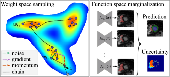
which, however, cannot be solved analytically without restrictive assumptions on the exact form of likelihood and prior model (e.g., Gaussian) (Gal and Ghahramani, 2016; Blei et al., 2017). We approximate the integration in Eq. eq:marginalization using the Monte-Carlo method, which is assumption-free and scalable to network sizes:
| (8) |
where are the samples drawn from the posterior distribution and is the voxel-wise probabilistic prediction made by the network with weight . In practice, the samples are saved checkpoints during the training or posterior sampling process and these samples can form an ensemble without the need to train multiple ensembles. Subsequently, we can estimate the predictive uncertainty map based on the voxel-wise binary entropy of each class or the categorical distribution entropy (Mehrtash et al., 2020):
| (9) | ||||
| (10) |
where .
2.3 Posterior Sampling via Hamiltonian Monte Carlo
HMC is an MCMC variant that can effectively generate samples conforming to a given distribution (Neal et al., 2011; Chen et al., 2014), scalable to high dimensionality (Speagle, 2019). In this section, we introduce the HMC sampling of the CP distribution defined in Eq. eq:cold_post.
2.3.1 Stochastic Gradient Hamiltonian Monte Carlo
We propose drawing samples from the CP Eq. eq:cold_post, by HMC (Neal et al., 2011) sampling. HMC builds a Markov chain by simulating the motion of the particles in an energy field at position with momentum . The particle dynamics is governed by the Hamiltonian, , in which the potential energy drives the particle to a low energy state (equivalently, the low loss region in the weight space). The auxiliary momentum term simulates the kinetic energy that makes the particle explore the low-energy surface. Without loss of generality, the mass can be set as the identity matrix.
The HMC dynamics simulation requires the evaluation of the full batch gradient (Neal et al., 2011). In practice, however, we only have access to the stochastic gradient estimated on a mini-batch of size :
| (11) |
where is defined in Eq. eq:loss_function and . The stochastic gradient estimation introduces additional noise of strength to the true gradient. In the presence of such noise, the stationary distribution of the HMC samples is no longer the target distribution (Chen et al., 2014).
To address this problem, we propose to use the Stochastic Gradient Hamiltonian Monte Carlo (SGHMC) (Chen et al., 2014), which introduces a friction term that compensates for the stochastic gradient noise and a Gaussian noise to the momentum update such that the dampening friction matches the noise level. In practice, the tempered posterior by in Eq. eq:cold_post leads to the Hamiltonian , and the gradient scales linearly to . The Markov chain can be simulated according to the discrete form of SGHMC:
| (12) |
where is the friction coefficient, is the step size of HMC simulation. Note that the momentum update rule in Eq. eq:sghmc_discrete is equivalent to the following form:
| (13) |
by multiplying on both sides and use to replace the original . The dynamics of in Eq. eq:sghmc_discrete yield samples whose stationary distribution is exactly . This can be strictly proven via the Fokker-Planck-Equation of the stationary distribution of SGHMC (Särkkä and Solin, 2019; Chen et al., 2014).
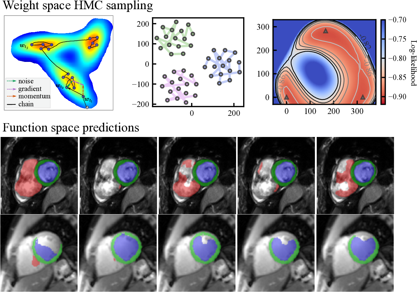
Here, we note that when , Eq. eq:sghmc_discrete is exactly the update rule of SGD with momentum, where is equivalent to the momentum term and is the learning rate. The length of the Markov chain is the number of iterations in network training using SGD-momentum. In this case, the single source of the stochastic noise is the gradient estimation noise in of strength . As increases, additional noise is injected and perturbs the gradient direction, which can be considered as an SGD-momentum process with elevated gradient estimation noise. In summary, the HMC sampling process is equivalent to the network optimization process as is shown in Eq. eq:sghmc_discrete and, thus, comes at no additional cost. The optimizer performs as a posterior sampler and the sampling process is in essence saving the checkpoints. The overview of the proposed method is shown in Fig. 1: the gradient (potential force) drives the chain to high-posterior-density regions, and the momentum term and the injected noise keep the chain exploring the vicinity of a local optimum.
2.3.2 Annealing Learning Rate and Sample Thinning
The learning rate controls the convergence in optimization and Monte Carlo sampling. We present a novel approach to reschedule the learning rate for more accurate posterior sampling. Specifically, to let the chain explore a broader area and prevent it from converging to a single point, we set the learning rate as a constant non-zero value after the fraction of the training budget. To capture the multimodal posterior geometry that is typical of complex DNNs (Zhang et al., 2019; Huang et al., 2017), we further propose to use cyclical annealing training such that the Markov chain can visit multiple modes of the posterior. We divide the training budget of epochs into cycles and each cycle consumes epochs. In particular, we propose to use a high learning rate at the beginning of each cycle such that the perturbation is strong enough to drive the chain into various posterior modes.
The overall learning rate for the Hamiltonian dynamics simulation is formulated as:
| (14) |
where is the intra-cycle epoch number and is the high restart learning rate which was set for the first epochs in each cycle.
The first fraction of training epochs are considered as the burn-in stage of SGHMC (Zhang et al., 2019). The weights computed at each iteration after the burn-in stage can be seen as a sample of the posterior distribution. However, a single iteration causes a marginal change in weights in the Markov chain, and the consecutive samples can be highly correlated. The auto-correlation between samples significantly reduces the number of effective samples in a Markov chain (Hammersley, 2013). Moreover, collecting all samples after the burn-in stage requires substantial disk space while the inference would be extremely time-consuming. After the burn-in stage, we, therefore, adopt the sample thinning strategy (Hammersley, 2013) to only collect samples at the end of every fourth epoch (every 1000 iterations): .
2.4 Weight and Functional Space Diversity
We differentiate two types of diversity for weights and function , respectively. Although both are relevant to uncertainty estimation, their relationship is complex and is largely understudied. To investigate the diversity of weights, we use mutual cosine similarity (Larrazabal et al., 2021) as a metric for weight space diversity, which is defined as:
| (15) |
Additionally, we monitor the volume of the high-dimensional space that the chain explored, via rectangular approximation:
| (16) |
where ’s are the first singular values of the matrix . In practice, we choose because the first five can explain at least of the total weight variance. Additionally, is a computationally practical choice because of the extremely high dimension of weights .
To investigate the diversity of functional space, we propose to evaluate the variation of predictions by on the validation set. Given two functions and , we measure the functional space distance on a validation set as:
| (17) |
where indicates where the ensemble prediction make erroneous predictions compared to the ground truth at voxel-level. We note that focusing only on such misclassified voxels can better manifest the difference between functions, because in practice, most of the voxels in an image are correctly classified (e.g., background), leading to an over-optimistically high agreement despite the diversity in organ segmentation.
2.5 Voxel-wise Calibration Metrics
To quantify the performance of voxel-wise calibration and uncertainty estimation, we use the Expected Calibration Error (ECE) (Guo et al., 2017), the Brier score (Br) (Brier et al., 1950) and the negative log-likelihood (NLL) (Ovadia et al., 2019). For a segmentation task with voxels in total, the confidence score ranging from to is equally divided into bins and the ECE score is defined as:
| (18) |
where is the set of voxels whose confidence falls into the bin, is the mean confidence and is the mean accuracy. The Brier score quantifies the deviation of predictive categorical distribution from the ground truth one-hot label:
| (19) |
and the NLL metric is defined as:
| (20) |
2.6 Image-level Confidence Score and Failure Detection
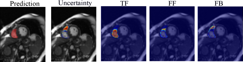
Based on the estimated entropy map, we aggregate the voxel-wise uncertainty and derive an image-level confidence score as a segmentation failure indicator. Specifically, we estimate the correct segmentation (true foreground, TF), the over-segmentation (false foreground, FF), and under-segmentation (false background, FB) areas as follows:
| (21) | ||||
where is the segmentation map for class and is the corresponding entropy map. The final confidence score of the generated segmentation map with uncertainty is given by simulating the Dice coefficient:
| (22) |
Examples of the estimated TF, FF, and FB maps are shown in Fig. 2. We detect possible failures based on the computed confidence score and measure the performance of image-level failure detection by the area under the receiver operating characteristic curve (AUC). Empirically, for cardiac MRI applications, a segmentation prediction on a 2D image slice with a dice score lower than 80% and an average symmetric surface distance (ASSD) greater than 2mm is considered a segmentation failure.
3 Experiments
3.1 Dataset
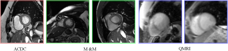
We evaluated the proposed HMC-CP method on nnU-Net (Isensee et al., 2021), an established U-Net architecture, for the cardiac MRI task. We use the ACDC dataset (Bernard et al., 2018) for training and validation, which consists of short-axis end-diastolic (ED) and end-systolic (ES) cardiac MRI steady-state free precession (SSFP) cine images of 100 subjects acquired at 1.5T (Aera, Siemens Healthineers, Erlangen, Germany) and 3T (Tim Trio, Siemens Healthineers, Erlangen Germany). The original training part of the dataset with 100 subjects was randomly split into a training set () and a validation set (). The validation set was used for selecting the best temperature and studying the influence of the number of samples on the segmentation and calibration performance. Based on the validation results, we evaluate our methods on the ACDC test set consisting of 50 subjects to test the in-domain performance. For out-of-domain performance, we tested the proposed method and other methods in comparison on a completely independent dataset, the Multi-center Multi-vendor (M&M) cardiac MRI (Campello et al., 2021), which contains 320 SSFP cine scans of end-systolic (ES) and end-diastolic (ED) images collected from 6 medical centers using different 1.5T -(Siemens Avanto, Germany, Philips Achieva, Netherlands; GE Signa Excite; and Cannon Vantage Orian); and 3T scanners (Siemens Skyra, Germany). Additionally, we also evaluate the proposed method on a quantitative MRI (QMRI) dataset, containing 112 modified look-locker inversion recovery (MOLLI) -mapping (Messroghli et al., 2004) images and -prep-based -mapping (Giri et al., 2009) images. The images are collected from 8 healthy subjects at 3T (Prisma, Siemens Healthineers, Erlangen, Germany). Each image contains several (8 for -mapping and 5 for T2-mapping) baseline images that were read out during the or relaxation processes. We show some exemplar images of the three datasets in Fig. 3. Three classes of ground truth labels are provided in the ACDC and M&M datasets: left ventricle cavity (LV), myocardium (MYO), and right ventricle (RV). For the QMRI dataset, the LV and MYO regions were manually annotated on the second baseline image which has relatively good contrast.
3.2 Methods in Comparison
We implemented several baseline methods including PHi-Seg (Baumgartner et al., 2019), Bayesian SegNet with Dropout (Kendall et al., 2015), Deep Ensembles (Lakshminarayanan et al., 2016; Mehrtash et al., 2020), and compared them to the proposed method in terms of both segmentation and uncertainty estimation. We used the automatically configured nnU-Net (Isensee et al., 2021) architecture, which is a commonly used reference for medical image segmentation. All methods were trained with epochs. We set the initial learning rate to be and used a fixed batch size of for all methods.
- •
PHi-Seg We implemented the PHi-Seg (Baumgartner et al., 2019) in the nnU-Net framework with resolution levels, latent levels and latent feature depth for the prior, likelihood and posterior networks. At inference time, we drew realizations of the hierarchical latent features from the prior network output and decoded the features with the likelihood network.
- •
MC-Dropout Following the Bayesian SegNet work (Kendall et al., 2015), we inserted dropout layers into the innermost three layers on both the encoder- and decoder-side of the U-Net. The dropout rate was set as at both the training and testing phases and we ran forward passes at test time.
- •
Deep Ensembles Deep Ensembles of 15 models were trained by SGD-momentum with random initialization for epochs with the standard exponential learning rate decay.
- •
SGHMC Variants We ran the proposed SGHMC method for cycles of epochs. In each cycle, the first fraction of each cycle was the burn-in stage. Afterward, the noise was injected into the momentum update. The noise level is controlled by the temperature as in Eq. eq:sghmc_discrete. To investigate the effect of cold posterior, we trained networks using SGHMC with temperature , where corresponds to SGD-momentum with constant learning rate (SGD-Const) (Zhao et al., 2022). The restart learning rate was set to and restarting epochs . The checkpoints were collected every epoch after the burn-in stage as posterior samples until the end of training. The weight evolution in the last training cycle was recorded for the single-mode sampling baselines (SGHMC-Single), and the checkpoints across all three modes form a set of multi-modal weight samples (SGHMC-Multi).
4 Results
4.1 Posterior Geometry and Chain Trajectory of SGHMC
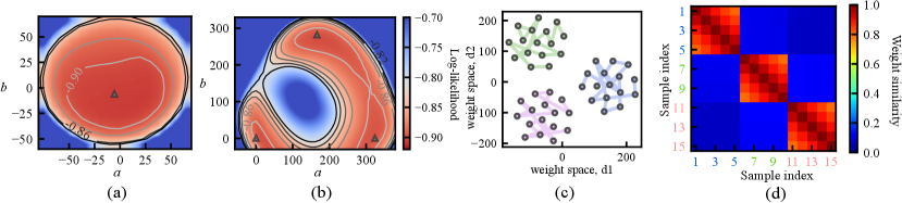
Fig. 1 (b) depicts the loss surface on the interpolated plane collected from three training cycles, illustrating the multi-modality of U-Net solution space. Via cyclical learning, the weight iterations visited multiple posterior modes, which can be observed from the t-SNE visualization of the training trajectory in Fig. 1 (c). Fig. 1 (d) visualizes the cosine similarity (Larrazabal et al., 2021) of checkpoints collected in three cycles which shows that the local weight checkpoints are similar to each other, while the cyclical training promotes the orthogonality of weights in different modes.
4.2 Diversity in Function Space
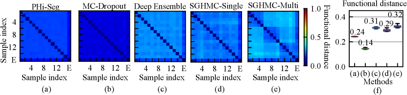
A high degree of diversity in the function space leads to better uncertainty estimation. We analyzed the functional diversity of all methods in comparison via evaluating the distance between function instances defined in Eq. eq:diversity_measure. The result is shown in Fig. 5 (a)-(e) as confusion matrices. The mutual diversity levels for all methods are summarised in Fig. 5 (f). We show that the PHi-Seg and MC-Dropout methods have lower functional diversity in the functional space compared to Deep Ensembles and the proposed HMC variants, namely SGHMC-Single and SGHMC-Multi. The SGHMC-Single model yielded slightly lower diversity than that of Deep Ensembles, however, the SGHMC-Multi model showed the highest diversity, surpassing Deep Ensembles.
4.3 The Effect of Cold Posterior
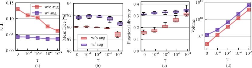
We also studied the effect of varying temperatures on the calibration and segmentation in both with or without augmentation cases. Fig. 6 (a) shows the calibration performance variation with an increasing temperature from to . From the figure, we observe that the model is not in favor of a cold posterior when augmentation is turned off, as the NLL consistently improves as the temperature increases from to . However, the NLL is relatively less sensitive to the changes in temperature when data augmentation is on and the NLL drop is relatively marginal compared with the without augmentation case. Fig. 6 (b) shows that the mean Dice across LV/MYO/RV drops in both cases as the temperature increases. We conjecture that this is because of the sampling on sub-optimal loss levels because of injected noise. The best segmentation accuracy is achieved at . Fig. 6 (c) - (d) reveals that higher temperature drives the chain to explore broader weight space because the weight volume increases exponentially with an increasing temperature. However, the functional diversity is more sensitive to the weight space volume change as is shown in Fig. 6 (c) when the augmentation is turned off. When the augmentation is on, we observe that a cold posterior at provides good calibration and improved segmentation performance. In the following, we use to evaluate our method on the test sets.
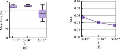
4.4 The Effect of Prior
In Fig. 7, we study the effect of varying prior strength defined in Eq. eq:loss_function. Smaller indicates a higher prior variance and thus a weaker prior assumption. From Fig. 7 (a) - (b), we observe that the stronger prior assumptions with cause a significant performance drop in Dice, but the calibration performance measured by NLL was improved. As the prior strength increases, its contribution to the posterior geometry is more pronounced and the likelihood part that fits the training data can end up with a sub-optimal level and thus lead to a lower accuracy. However, smaller prior can cause a slight performance drop compared with , which shows that a proper regularization is beneficial to the accuracy.
4.5 Calibration and Segmentation Performance
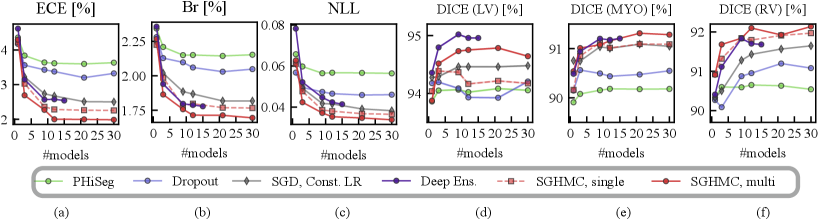
In Fig. 8, we show the calibration quality and segmentation performance as a function of , which is the number of models (predictions) averaged on the in-distribution validation set. The figure shows that the segmentation performance of the PHi-Seg framework is not competitive with other methods of comparison. Ensembling consistently improves the segmentation performance for all methods, however, the segmentation performance improvement via ensembling MC-Dropout and PHi-Seg predictions is relatively marginal compared to Deep Ensembles and HMC, in accordance with our finding that PHi-Seg and MC-Dropout lack functional diversity. On the in-distribution validation set, an ensemble of cyclical SGHMC (SGHMC-Multi) samples achieved the best performance. Fig. 8 (a)-(c) list the calibration results measured by ECE, Brier score, and NLL respectively. From the figures, we observe that a single model has poor calibration for all methods in comparison while combining more predictions consistently improves the model calibration. MC-Dropout improves calibration but is not as good as the ensemble of SGHMC with a constant learning rate (SGD-Const) at . Compared with SGD-Const (), SGHMC-Single () achieved better calibration performance, which was further surpassed by SGHMC-Multi, which ensembles from multiple posterior modes.
| Methods | ACDC | M&M | QMRI | |||||
|---|---|---|---|---|---|---|---|---|
| LV | MYO | RV | LV | MYO | RV | LV | MYO | |
| Vanilla (M=1) | 92.80±5.15 | 87.03±3.65 | 90.08±5.71 | 88.64±7.75 | 82.97±5.49 | 86.34±9.36 | 74.17±38.45 | 63.88±31.51 |
| PhiSeg (M=30) | 93.64±3.81 | 87.84±3.50 | 88.47±7.32 | 89.79±8.11 | 84.05±5.60 | 84.83±11.16 | 87.11±25.87 | 74.59±21.77 |
| Dropout (M=30) | 93.36±4.41 | 87.47±3.66 | 89.50±6.55 | 90.19±6.49 | 83.30±5.45 | 86.45±9.16 | 85.44±28.08 | 72.51±23.96 |
| Deep Ens. (M=30) | 93.84±3.79 | 87.91±3.54 | 90.92±5.39 | 90.13±6.96 | 84.48±5.25 | 87.43±8.53 | 82.31±31.52 | 70.29±27.04 |
| SGD Const. LR (M=30) | 93.70±4.27 | 87.97±3.57 | 90.61±5.88 | 90.28±6.71 | 84.21±5.14 | 87.26±9.80 | 85.77±27.38 | 73.11±23.80 |
| SGHMC, single (M=30) | 93.54±5.13 | 87.91±3.45 | 90.16±6.65 | 90.48±6.64 | 84.21±5.26 | 87.40±8.98 | 86.31±26.11 | 74.22±22.27 |
| SGHMC, multi (M=30) | 93.88±3.82 | 87.97±3.65 | 90.74±5.79 | 90.31±6.88 | 84.43±5.22 | 87.38±9.03 | 89.88±20.30 | 76.20±19.16 |
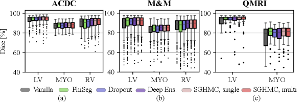
The segmentation performance measured by Dice score is listed in Fig. 9 and Table 1. The results show that the proposed method improves segmentation performance compared to the Vanilla model on all test sets. This indicates that Bayesian inference via averaging posterior samples leads to more accurate prediction. On the ACDC test set and M&M, the performance of Deep Ensemble and the proposed method are marginally better than other methods in comparison. There is little difference between the segmentation performance of the single-modal and multi-modal variants of the proposed model. Additionally, we observe that there exists little difference between the proposed method and traditional methods like Deep Ensembles. However, it is not our primary purpose to significantly increase the segmentation performance against the traditional methods. Instead, we are more interested in the calibration and uncertainty quantification performance.
The results also show that domain shifts cause a performance drop, but our proposed method by marginalizing HMC samples is more robust to the contrast changes. Comparing the results on the three datasets, we observe a drastic performance drop as the domain shift increases from cine (ACDC, M&M) to QMRI. The MYO Dice of the vanilla model drops from to on QMRI. However, on the QMRI dataset with the largest domain shift, the proposed method exhibits high robustness and achieved the highest Dice score on both LV () and MYO ().
| Methods | ACDC | M&M | QMRI | ||||||
|---|---|---|---|---|---|---|---|---|---|
| ECE[%] | Br [%] | NLL[%] | ECE [%] | Br [%] | NLL [%] | ECE [%] | Br [%] | NLL[%] | |
| Vanilla (M=1) | 5.45±1.63 | 2.76±0.80 | 9.45±3.87 | 6.49±2.81 | 3.28±1.40 | 11.96±7.25 | 29.66±25.39 | 14.92±12.65 | 76.01±83.30 |
| PhiSeg (M=30) | 4.55±1.86 | 2.61±0.96 | 6.91±3.94 | 5.55±2.82 | 3.11±1.44 | 8.68±5.55 | 14.87±18.65 | 8.03±9.16 | 28.23±48.75 |
| Dropout (M=30) | 5.09±1.71 | 2.69±0.87 | 8.10±3.49 | 6.19±2.50 | 3.23±1.29 | 10.66±5.75 | 22.79±19.06 | 11.60±9.10 | 42.03±47.43 |
| Deep Ens. (M=15) | 3.49±1.20 | 2.20±0.63 | 5.55±2.01 | 4.49±2.14 | 2.71±1.12 | 7.51±4.35 | 20.67±19.94 | 10.73±9.33 | 28.61±37.71 |
| SGD Const. LR (M=30) | 3.68±1.40 | 2.27±0.70 | 5.38±1.93 | 4.81±2.35 | 2.81±1.24 | 7.65±4.64 | 19.92±18.65 | 10.35±8.98 | 26.91±33.44 |
| SGHMC, single (M=30) | 3.54±1.23 | 2.24±0.64 | 5.17±1.68 | 4.75±2.23 | 2.81±1.19 | 7.43±4.21 | 20.11±17.11 | 10.33±8.03 | 26.11±27.29 |
| SGHMC, multi (M=30) | 3.29±1.18 | 2.19±0.63 | 4.89±1.53 | 4.38±2.19 | 2.72±1.17 | 6.91±4.00 | 19.81±15.60 | 10.18±7.56 | 25.16±24.91 |
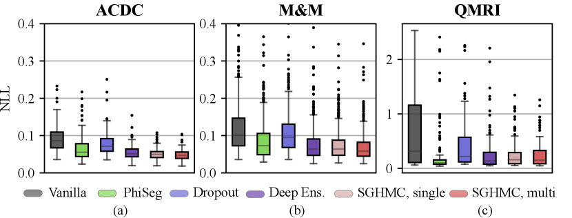
In Fig. 10 and Table 2, we report the voxel-wise calibration metrics of methods in comparison. The figure and table show that the calibration performance decreases consistently as the domain shift becomes larger. Overall, the multi-modal SGHMC predictions deliver the best calibration performance, significantly better than baseline methods like MC-Dropout and Phi-Seg on the cine datasets (ACDC and M&M). This is in accordance with the results in Sec. 4.2 which show that the HMC samples have higher functional diversity. On the QMRI dataset, the PhiSeg network achieved the best ECE and Brier score, but the single-modal and multi-modal SGHMC variants have the lowest NLL. Comparing the results of Dropout and Deep Ensemble, the proposed method is robustly well-calibrated even in the presence of a large domain shift.
4.6 Automated Failure Detection
| Methods | ACDC | M&M | QMRI | |||||
|---|---|---|---|---|---|---|---|---|
| LV | MYO | RV | LV | MYO | RV | LV | MYO | |
| Vanilla | 73.54 | 83.43 | 69.80 | 85.67 | 88.69 | 79.56 | 22.22 | 37.04 |
| PhiSeg | 59.41 | 60.05 | 65.88 | 71.02 | 71.31 | 74.10 | 22.01 | 43.58 |
| Dropout | 92.35 | 96.99 | 84.57 | 87.23 | 89.23 | 84.94 | 62.47 | 70.75 |
| Deep Ens. | 93.21 | 96.42 | 84.57 | 88.43 | 90.71 | 85.93 | 93.68 | 89.41 |
| SGHMC, single | 91.49 | 97.27 | 88.20 | 88.31 | 91.08 | 86.98 | 86.83 | 91.47 |
| SGHMC, multi | 91.12 | 95.54 | 88.21 | 89.33 | 92.05 | 86.70 | 92.88 | 89.20 |
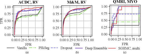
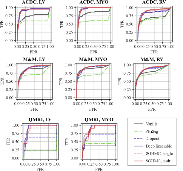
With the proposed image-level uncertainty score, we could automatically detect segmentation failure for the test datasets. Table 3 lists the AUC values of failure detection on three datasets. MC-Dropout, deep ensemble, and the proposed HMC variants achieved similar performances in failure detection of LV and MYO segmentations on the ACDC dataset. However, the proposed method can detect segmentation failure of the most challenging anatomy RV better with an AUC of 88.21%, which is higher than deep ensemble (84.57%) and MC-Dropout (84.57%). This is also reflected in the ROC curve in Fig. 11 (a) which shows that the ROC of the proposed method encloses that of Deep Ensemble and MC-Dropout. The improvement is also observed in M&M and QMRI datasets. The proposed method achieved a remarkable AUC (91.47%) on the QMRI dataset, significantly outperforming the MC-Dropout(70.75%). Despite the good voxel-wise calibration, PHi-Seg suffers from severe silent failures on QMRI with an AUC of 43.58%. More detailed ROC curves are listed in Appendix A, Fig. 15.
4.7 Qualitative Results
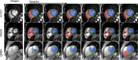
Fig. 12 visualizes the segmentation predictions made by HMC samples. From the figure, we can observe a consistency across these predictions on a certain input, for example, on the cine case from the ACDC dataset. However, on uncertain inputs like the M&M cine case, the samples tend to make diverse predictions on the RV basal areas. As the contrast change increases further, the network also makes different predictions on the LV blood pool and myocardium because of the low contrast of QMRI images.
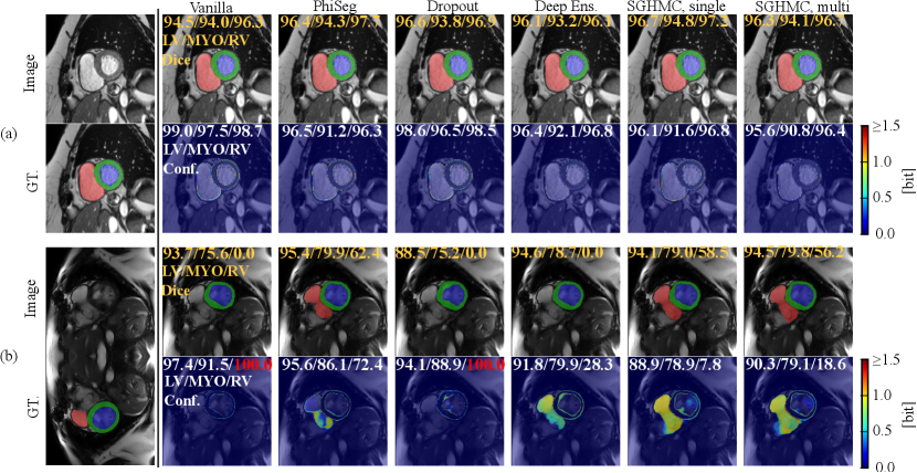
In Fig. 13, we visualize the predictions on the cine images and estimated uncertainty maps produced by all methods in comparison. Fig. 13 (a) depicts a middle slice image on which all the methods make accurate predictions and the uncertainty concentrates only on the border between anatomical structures. However, in all four cases, the vanilla network can only output high uncertainty on the border area, even in the presence of erroneous predictions (i.e. silent failure). In general, for cardiac MRI segmentation tasks, uncertainty, and segmentation failure occur more frequently on the right ventricle. A typical failure case is shown in Figure. 13 (b), on which the Phi-Seg outputs zero uncertainty on RV voxels.
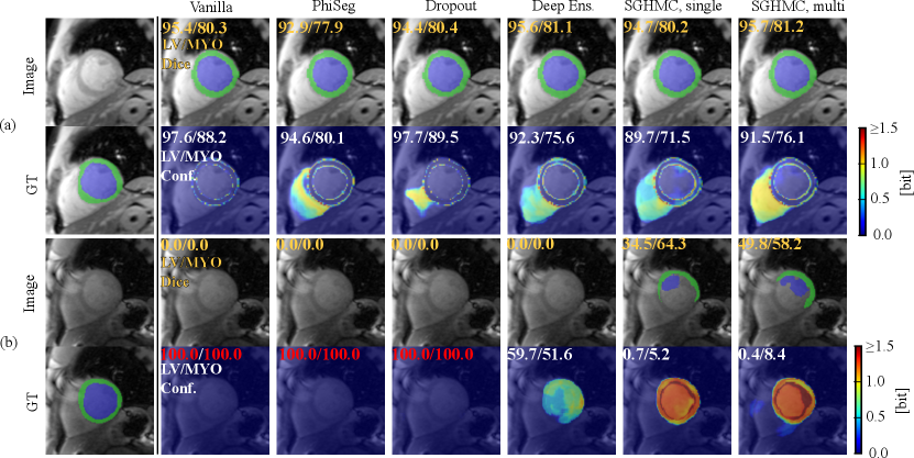
Figure. 14 (a) shows a QMRI image case on which the network successfully segmented MYO and LV, and a high level of confidence scores are provided by all the methods. Fig. 14 (b) depicts the uncertainty estimation results on a hard QMRI image. Under the strong domain shift, PHiSeg and MC-Dropout failed to detect the segmentation failures. In all cases, our proposed HMC variants demonstrated much better uncertainty estimation performance, without the risk of “silent failures”.
5 Discussion and Conclusion
DL models have achieved extraordinary performance for medical image segmentation tasks. However, they are generally miscalibrated and can fail silently. This seriously undermines DL models’ trustworthiness in clinical utilization. In this work, we propose a framework of Bayesian deep learning for uncertainty estimation and failure detection for DL-based medical image segmentation.
To make the high-dimensional Bayesian segmentation problem computationally tractable, we formulated it as a posterior sampling problem, which can be solved by HMC. Diversity in the functional space plays a critical role in uncertainty estimation. We have shown that, in the context of cardiac MRI segmentation, the HMC can effectively produce network samples that make diverse segmentation predictions with a thinning of 4 epochs in our practice. Moreover, ensembling more than samples in one chain simulation can provide comparable or even superior performance compared to training deep ensemble models. Comparing the functional diversity of various methods, we observe that degraded calibration performance strongly correlates with the lack of functional diversity. HMC samples and Deep Ensembles can produce functions of high diversity and their calibration is also superior to other methods including PHi-Seg and MC-Dropout.
We also noticed that cold posterior (CP) is crucial to an accurate and well-calibrated prediction for segmentation purposes. Specifically, we observe that HMC at temperature forms an outstanding baseline for model calibration. This method is also successfully validated on the segmentation of shapes with multiple connected components like lymph nodes (Salahuddin et al., 2023). Moreover, the performance can be further improved by increasing to a cold temperature at . On the other hand, when the data augmentation is turned off, a cold temperature causes a significant drop in model calibration.
In general, the marginalization of diverse functions is beneficial to the segmentation accuracy. All methods improve the segmentation accuracy by combining predictions made by various network samples. A relatively higher function space diversity improves the segmentation accuracy, comparing HMC to PHi-Seg and MC-Dropout. However, overly high function space diversity could harm the segmentation accuracy. HMC with a higher temperature produces an elevated level of functional diversity but the segmentation accuracy drops. In contrast, the calibration consistently improves with an increasing temperature.
In particular, our proposed method has addressed the two major issues of current Bayesian learning methods for large, over-parameterized neural networks. First, it makes no restrictive assumptions on weight posterior as the VI family of Bayesian methods (including the VI proxy such as MC Dropout). Second, with our proposed cyclical annealing strategy, the method is highly computationally efficient, only consuming the same computation budget as a single-round standard network training. The resemblance between HMC and SGD with momentum makes posterior sampling as straightforward as saving checkpoints during network training. Nonetheless, we acknowledge that with more computational resources, Deep Ensembles can also be trained in parallel, which is also time-efficient and further enables combining predictions from various network architectures. We did not cover the ensembling of different architectures in our work, which we see as a limitation. However, our method still forms an outstanding baseline with less training effort and energy consumption.
In practice, HMC parameters like batch size and learning rate can directly affect the simulation (training) dynamics, because the batch size determines the strength of the gradient estimation noise and the learning rate controls the range of exploration. We used a radical learning rate to promote diversity but the influence of batch size and learning rate on the final performance has not been fully discussed. We see this as a limitation and an interesting future work direction.
By the proposed image-level confidence score, we can also automatically detect the possible segmentation failure on each image. We showed that the automatic failure detection is highly robust on both in-domain cine images and QMRI images with a strong domain shift with AUC above . The HMC approach is especially robust to large domain shifts like cine to QMRI, being the most robust one to detect myocardial segmentation failure in quantitative CMR with an AUC of . When integrated into the DL workflow, automatic failure detection potentially improves the trustworthiness of DL models deployed on large-scale clinical studies or in daily clinical practice.
In conclusion, we have proposed a Bayesian learning framework for uncertainty estimation of medical image segmentation, by Hamiltonian Monte Carlo with cold posterior (HMC-CP). HMC-CP is theoretically grounded, computationally efficient, and scalable to large medical image segmentation networks. Our extensive experiments on both in-domain and out-of-domain data showed that the proposed HMC-CP method results in more reliable uncertainty estimation, as well as more accurate image segmentation, compared with a range of state-of-the-art baselines. Importantly, by reliable uncertainty estimation, our method provides a promising direction for improving the trustworthiness of DL models in clinical applications.
Acknowledgments
YZ and QT acknowledge the TU Delft AI Initiative for financial support, and the NVIDIA Applied Research Accelerator Program for granting high-performance computing resources. JT and SW are supported by the NWO Start-up grant STU.019.024, the TU Delft - Erasmus MC Convergence Impulse initiative, the European Union (ERC, Vascular ID, 101078711), and the Netherlands Heart Foundation Dekker Grant. TAT is supported by the British Heart Foundation (IRF FS/19/35/34374). IP and TAT are directly and indirectly supported by the University College London Hospitals NIHR Biomedical Research Centre and Biomedical Research Unit at Barts Hospital respectively.
Ethical Standards
The work follows appropriate ethical standards in conducting research and writing the manuscript, following all applicable laws and regulations regarding the treatment of animals or human subjects.
Conflicts of Interest
We declare we don’t have conflicts of interest.
References
- Abdar et al. (2021) Moloud Abdar, Farhad Pourpanah, Sadiq Hussain, Dana Rezazadegan, Li Liu, Mohammad Ghavamzadeh, Paul Fieguth, Xiaochun Cao, Abbas Khosravi, U Rajendra Acharya, et al. A review of uncertainty quantification in deep learning: Techniques, applications and challenges. Information Fusion, 76:243–297, 2021.
- Baumgartner et al. (2019) Christian F Baumgartner, Kerem C Tezcan, Krishna Chaitanya, Andreas M Hötker, Urs J Muehlematter, Khoschy Schawkat, Anton S Becker, Olivio Donati, and Ender Konukoglu. Phiseg: Capturing uncertainty in medical image segmentation. In International Conference on Medical Image Computing and Computer-Assisted Intervention, pages 119–127. Springer, 2019.
- Bernard et al. (2018) Olivier Bernard, Alain Lalande, Clement Zotti, Frederick Cervenansky, Xin Yang, Pheng-Ann Heng, Irem Cetin, Karim Lekadir, Oscar Camara, Miguel Angel Gonzalez Ballester, et al. Deep learning techniques for automatic mri cardiac multi-structures segmentation and diagnosis: is the problem solved? IEEE transactions on medical imaging, 37(11):2514–2525, 2018.
- Blei et al. (2017) David M Blei, Alp Kucukelbir, and Jon D McAuliffe. Variational inference: A review for statisticians. Journal of the American statistical Association, 112(518):859–877, 2017.
- Blundell et al. (2015) Charles Blundell, Julien Cornebise, Koray Kavukcuoglu, and Daan Wierstra. Weight uncertainty in neural network. In International Conference on Machine Learning, pages 1613–1622. PMLR, 2015.
- Brier et al. (1950) Glenn W Brier et al. Verification of forecasts expressed in terms of probability. Monthly weather review, 78(1):1–3, 1950.
- Campello et al. (2021) Víctor M Campello, Polyxeni Gkontra, Cristian Izquierdo, Carlos Martín-Isla, Alireza Sojoudi, Peter M Full, Klaus Maier-Hein, Yao Zhang, Zhiqiang He, Jun Ma, et al. Multi-centre, multi-vendor and multi-disease cardiac segmentation: the m&ms challenge. IEEE Transactions on Medical Imaging, 40(12):3543–3554, 2021.
- Carvalho et al. (2020) Eduardo DC Carvalho, Ronald Clark, Andrea Nicastro, and Paul HJ Kelly. Scalable uncertainty for computer vision with functional variational inference. In Proceedings of the IEEE/CVF Conference on Computer Vision and Pattern Recognition, pages 12003–12013, 2020.
- Chen et al. (2020) Chen Chen, Chen Qin, Huaqi Qiu, Giacomo Tarroni, Jinming Duan, Wenjia Bai, and Daniel Rueckert. Deep learning for cardiac image segmentation: a review. Frontiers in Cardiovascular Medicine, 7:25, 2020.
- Chen et al. (2014) Tianqi Chen, Emily Fox, and Carlos Guestrin. Stochastic gradient hamiltonian monte carlo. In International conference on machine learning, pages 1683–1691. PMLR, 2014.
- (11) P. Chlap, H. Min, N. Vandenberg, J. Dowling, L. Holloway, and A. Haworth. A review of medical image data augmentation techniques for deep learning applications. Journal of Medical Imaging and Radiation Oncology.
- Czolbe et al. (2021) Steffen Czolbe, Kasra Arnavaz, Oswin Krause, and Aasa Feragen. Is segmentation uncertainty useful? In Information Processing in Medical Imaging: 27th International Conference, IPMI 2021, Virtual Event, June 28–June 30, 2021, Proceedings 27, pages 715–726. Springer, 2021.
- Der Kiureghian and Ditlevsen (2009) Armen Der Kiureghian and Ove Ditlevsen. Aleatory or epistemic? does it matter? Structural safety, 31(2):105–112, 2009.
- Folgoc et al. (2021) Loic Le Folgoc, Vasileios Baltatzis, Sujal Desai, Anand Devaraj, Sam Ellis, Octavio E Martinez Manzanera, Arjun Nair, Huaqi Qiu, Julia Schnabel, and Ben Glocker. Is mc dropout bayesian? arXiv preprint arXiv:2110.04286, 2021.
- Fort et al. (2019) Stanislav Fort, Huiyi Hu, and Balaji Lakshminarayanan. Deep ensembles: A loss landscape perspective. arXiv preprint arXiv:1912.02757, 2019.
- Gal and Ghahramani (2016) Yarin Gal and Zoubin Ghahramani. Dropout as a bayesian approximation: Representing model uncertainty in deep learning. In international conference on machine learning, pages 1050–1059. PMLR, 2016.
- Gao et al. (2023) Shangqi Gao, Hangqi Zhou, Yibo Gao, and Xiahai Zhuang. Bayeseg: Bayesian modeling for medical image segmentation with interpretable generalizability. arXiv preprint arXiv:2303.01710, 2023.
- Garipov et al. (2018) Timur Garipov, Pavel Izmailov, Dmitrii Podoprikhin, Dmitry P Vetrov, and Andrew G Wilson. Loss surfaces, mode connectivity, and fast ensembling of dnns. Advances in neural information processing systems, 31, 2018.
- Giri et al. (2009) Shivraman Giri, Yiu-Cho Chung, Ali Merchant, Georgeta Mihai, Sanjay Rajagopalan, Subha V Raman, and Orlando P Simonetti. T2 quantification for improved detection of myocardial edema. Journal of cardiovascular magnetic resonance, 11(1):1–13, 2009.
- Gonzalez and Mukhopadhyay (2021) Camila Gonzalez and Anirban Mukhopadhyay. Self-supervised out-of-distribution detection for cardiac cmr segmentation. In Medical Imaging with Deep Learning, 2021.
- Gonzalez et al. (2021) Camila Gonzalez, Karol Gotkowski, Andreas Bucher, Ricarda Fischbach, Isabel Kaltenborn, and Anirban Mukhopadhyay. Detecting when pre-trained nnu-net models fail silently for covid-19 lung lesion segmentation. In International Conference on Medical Image Computing and Computer-Assisted Intervention, pages 304–314. Springer, 2021.
- Guo et al. (2017) Chuan Guo, Geoff Pleiss, Yu Sun, and Kilian Q Weinberger. On calibration of modern neural networks. In International Conference on Machine Learning, pages 1321–1330. PMLR, 2017.
- Gustafsson et al. (2020) Fredrik K Gustafsson, Martin Danelljan, and Thomas B Schon. Evaluating scalable bayesian deep learning methods for robust computer vision. In Proceedings of the IEEE/CVF conference on computer vision and pattern recognition workshops, pages 318–319, 2020.
- Hammam et al. (2021) Ahmed Hammam, Seyed Eghbal Ghobadi, Frank Bonarens, and Christoph Stiller. Real-time uncertainty estimation based on intermediate layer variational inference. In Proceedings of the 5th ACM Computer Science in Cars Symposium, pages 1–9, 2021.
- Hammersley (2013) John Hammersley. Monte carlo methods. Springer Science & Business Media, 2013.
- Hastings (1970) W Keith Hastings. Monte carlo sampling methods using markov chains and their applications. 1970.
- Hora (1996) Stephen C Hora. Aleatory and epistemic uncertainty in probability elicitation with an example from hazardous waste management. Reliability Engineering & System Safety, 54(2-3):217–223, 1996.
- Huang et al. (2017) Gao Huang, Yixuan Li, Geoff Pleiss, Zhuang Liu, John E Hopcroft, and Kilian Q Weinberger. Snapshot ensembles: Train 1, get m for free. arXiv preprint arXiv:1704.00109, 2017.
- Hüllermeier and Waegeman (2021) Eyke Hüllermeier and Willem Waegeman. Aleatoric and epistemic uncertainty in machine learning: An introduction to concepts and methods. Machine Learning, 110(3):457–506, 2021.
- Isensee et al. (2021) Fabian Isensee, Paul F Jaeger, Simon AA Kohl, Jens Petersen, and Klaus H Maier-Hein. nnu-net: a self-configuring method for deep learning-based biomedical image segmentation. Nature methods, 18(2):203–211, 2021.
- Izmailov et al. (2018) Pavel Izmailov, Dmitrii Podoprikhin, Timur Garipov, Dmitry Vetrov, and Andrew Gordon Wilson. Averaging weights leads to wider optima and better generalization. arXiv preprint arXiv:1803.05407, 2018.
- Izmailov et al. (2021) Pavel Izmailov, Sharad Vikram, Matthew D Hoffman, and Andrew Gordon Gordon Wilson. What are bayesian neural network posteriors really like? In International conference on machine learning, pages 4629–4640. PMLR, 2021.
- Jospin et al. (2022) Laurent Valentin Jospin, Hamid Laga, Farid Boussaid, Wray Buntine, and Mohammed Bennamoun. Hands-on bayesian neural networks—a tutorial for deep learning users. IEEE Computational Intelligence Magazine, 17(2):29–48, 2022.
- Jungo and Reyes (2019) Alain Jungo and Mauricio Reyes. Assessing reliability and challenges of uncertainty estimations for medical image segmentation. In International Conference on Medical Image Computing and Computer-Assisted Intervention, pages 48–56. Springer, 2019.
- Jungo et al. (2020) Alain Jungo, Fabian Balsiger, and Mauricio Reyes. Analyzing the quality and challenges of uncertainty estimations for brain tumor segmentation. Frontiers in neuroscience, page 282, 2020.
- Kapoor et al. (2022) Sanyam Kapoor, Wesley J Maddox, Pavel Izmailov, and Andrew Gordon Wilson. On uncertainty, tempering, and data augmentation in bayesian classification. arXiv preprint arXiv:2203.16481, 2022.
- Kendall and Gal (2017) Alex Kendall and Yarin Gal. What uncertainties do we need in bayesian deep learning for computer vision? Advances in neural information processing systems, 30, 2017.
- Kendall et al. (2015) Alex Kendall, Vijay Badrinarayanan, and Roberto Cipolla. Bayesian segnet: Model uncertainty in deep convolutional encoder-decoder architectures for scene understanding. arXiv preprint arXiv:1511.02680, 2015.
- Kohl et al. (2018) Simon AA Kohl, Bernardino Romera-Paredes, Clemens Meyer, Jeffrey De Fauw, Joseph R Ledsam, Klaus H Maier-Hein, SM Eslami, Danilo Jimenez Rezende, and Olaf Ronneberger. A probabilistic u-net for segmentation of ambiguous images. arXiv preprint arXiv:1806.05034, 2018.
- Lakshminarayanan et al. (2016) Balaji Lakshminarayanan, Alexander Pritzel, and Charles Blundell. Simple and scalable predictive uncertainty estimation using deep ensembles. arXiv preprint arXiv:1612.01474, 2016.
- Lampinen and Vehtari (2001) Jouko Lampinen and Aki Vehtari. Bayesian approach for neural networks—review and case studies. Neural networks, 14(3):257–274, 2001.
- Larrazabal et al. (2021) Agostina J Larrazabal, César Martínez, Jose Dolz, and Enzo Ferrante. Orthogonal ensemble networks for biomedical image segmentation. In International Conference on Medical Image Computing and Computer-Assisted Intervention, pages 594–603. Springer, 2021.
- Lifshitz and Landau (1984) EM Lifshitz and Lev Davidovich Landau. Statistical physics (course of theoretical physics, volume 5), 1984.
- MacKay (1995) David JC MacKay. Bayesian neural networks and density networks. Nuclear Instruments and Methods in Physics Research Section A: Accelerators, Spectrometers, Detectors and Associated Equipment, 354(1):73–80, 1995.
- Maddox et al. (2019) Wesley J Maddox, Pavel Izmailov, Timur Garipov, Dmitry P Vetrov, and Andrew Gordon Wilson. A simple baseline for bayesian uncertainty in deep learning. Advances in Neural Information Processing Systems, 32, 2019.
- Marcot and Penman (2019) Bruce G Marcot and Trent D Penman. Advances in bayesian network modelling: Integration of modelling technologies. Environmental modelling & software, 111:386–393, 2019.
- Mehrtash et al. (2020) Alireza Mehrtash, William M Wells, Clare M Tempany, Purang Abolmaesumi, and Tina Kapur. Confidence calibration and predictive uncertainty estimation for deep medical image segmentation. IEEE transactions on medical imaging, 39(12):3868–3878, 2020.
- Messroghli et al. (2004) Daniel R Messroghli, Aleksandra Radjenovic, Sebastian Kozerke, David M Higgins, Mohan U Sivananthan, and John P Ridgway. Modified look-locker inversion recovery (molli) for high-resolution t1 mapping of the heart. Magnetic Resonance in Medicine: An Official Journal of the International Society for Magnetic Resonance in Medicine, 52(1):141–146, 2004.
- Minderer et al. (2021) Matthias Minderer, Josip Djolonga, Rob Romijnders, Frances Hubis, Xiaohua Zhai, Neil Houlsby, Dustin Tran, and Mario Lucic. Revisiting the calibration of modern neural networks. Advances in Neural Information Processing Systems, 34:15682–15694, 2021.
- Mingard et al. (2021) Chris Mingard, Guillermo Valle-Pérez, Joar Skalse, and Ard A Louis. Is sgd a bayesian sampler? well, almost. Journal of Machine Learning Research, 22, 2021.
- Nabarro et al. (2021) Seth Nabarro, Stoil Ganev, Adria Garriga-Alonso, Vincent Fortuin, Mark van der Wilk, and Laurence Aitchison. Data augmentation in bayesian neural networks and the cold posterior effect. arXiv preprint arXiv:2106.05586, 2021.
- Neal (2012) Radford M Neal. Bayesian learning for neural networks, volume 118. Springer Science & Business Media, 2012.
- Neal et al. (2011) Radford M Neal et al. Mcmc using hamiltonian dynamics. Handbook of markov chain monte carlo, 2(11):2, 2011.
- Ouyang et al. (2022) Cheng Ouyang, Shuo Wang, Chen Chen, Zeju Li, Wenjia Bai, Bernhard Kainz, and Daniel Rueckert. Improved post-hoc probability calibration for out-of-domain mri segmentation. In International Workshop on Uncertainty for Safe Utilization of Machine Learning in Medical Imaging, pages 59–69. Springer, 2022.
- Ovadia et al. (2019) Yaniv Ovadia, Emily Fertig, Jie Ren, Zachary Nado, David Sculley, Sebastian Nowozin, Joshua V Dillon, Balaji Lakshminarayanan, and Jasper Snoek. Can you trust your model’s uncertainty? evaluating predictive uncertainty under dataset shift. arXiv preprint arXiv:1906.02530, 2019.
- Risten (1989) H Risten. The fokker-planck equation: methods of solution and applications. Springer Series in Synergetics, 18:544–3, 1989.
- Ronneberger et al. (2015) Olaf Ronneberger, Philipp Fischer, and Thomas Brox. U-net: Convolutional networks for biomedical image segmentation. In International Conference on Medical image computing and computer-assisted intervention, pages 234–241. Springer, 2015.
- Salahuddin et al. (2023) Zohaib Salahuddin, Yi Chen, Xian Zhong, Henry C Woodruff, Nastaran Mohammadian Rad, Shruti Atul Mali, and Philippe Lambin. From head and neck tumour and lymph node segmentation to survival prediction on pet/ct: An end-to-end framework featuring uncertainty, fairness, and multi-region multi-modal radiomics. Cancers, 15(7):1932, 2023.
- Särkkä and Solin (2019) Simo Särkkä and Arno Solin. Applied stochastic differential equations, volume 10. Cambridge University Press, 2019.
- Speagle (2019) Joshua S Speagle. A conceptual introduction to markov chain monte carlo methods. arXiv preprint arXiv:1909.12313, 2019.
- Wang et al. (2021) Deng-Bao Wang, Lei Feng, and Min-Ling Zhang. Rethinking calibration of deep neural networks: Do not be afraid of overconfidence. Advances in Neural Information Processing Systems, 34:11809–11820, 2021.
- Wang et al. (2019) Guotai Wang, Wenqi Li, Michael Aertsen, Jan Deprest, Sébastien Ourselin, and Tom Vercauteren. Aleatoric uncertainty estimation with test-time augmentation for medical image segmentation with convolutional neural networks. Neurocomputing, 338:34–45, 2019.
- Wang and Yeung (2020) Hao Wang and Dit-Yan Yeung. A survey on bayesian deep learning. ACM Computing Surveys (CSUR), 53(5):1–37, 2020.
- Wenzel et al. (2020) Florian Wenzel, Kevin Roth, Bastiaan S Veeling, Jakub Swiatkowski, Linh Tran, Stephan Mandt, Jasper Snoek, Tim Salimans, Rodolphe Jenatton, and Sebastian Nowozin. How good is the bayes posterior in deep neural networks really? arXiv preprint arXiv:2002.02405, 2020.
- Yan et al. (2020) W. Yan, L. Huang, L. Xia, S. Gu, and Q. Tao. Mri manufacturer shift and adaptation: Increasing the generalizability of deep learning segmentation for mr images acquired with different scanners. 2020.
- Yan et al. (2019) Wenjun Yan, Yuanyuan Wang, Shengjia Gu, Lu Huang, Fuhua Yan, Liming Xia, and Qian Tao. The domain shift problem of medical image segmentation and vendor-adaptation by unet-gan. In Medical Image Computing and Computer Assisted Intervention–MICCAI 2019: 22nd International Conference, Shenzhen, China, October 13–17, 2019, Proceedings, Part II 22, pages 623–631. Springer, 2019.
- Zhang et al. (2019) Ruqi Zhang, Chunyuan Li, Jianyi Zhang, Changyou Chen, and Andrew Gordon Wilson. Cyclical stochastic gradient mcmc for bayesian deep learning. arXiv preprint arXiv:1902.03932, 2019.
- Zhao et al. (2022) Yidong Zhao, Changchun Yang, Artur Schweidtmann, and Qian Tao. Efficient bayesian uncertainty estimation for nnu-net. In International Conference on Medical Image Computing and Computer-Assisted Intervention, pages 535–544. Springer, 2022.
A Detailed evaluation results