

1 Introduction
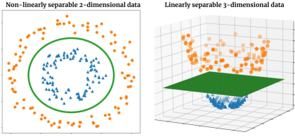
Support vector machines (SVMs) and other kernel based methods ushered in a new wave of supervised learning methods based on the fundamental insight that challenging tasks in low dimensions may become easier when the data is lifted to higher dimensional spaces (Boser et al., 1992; Cortes and Vapnik, 1995; Hofmann et al., 2008), as illustrated in Figure 1. These methods, however, become prohibitive when dealing with massive datasets in high dimensional feature spaces as their space complexity grows at least quadratically with the number of data points (Bordes et al., 2005; Novikov et al., 2016). Further, SVMs are also known to be sensitive to the specific choice of the kernel parameters and as a consequence the decision boundaries learnt are prone to over-fitting (Burges, 1998; Bordes et al., 2005). These factors have discouraged their successful adoption to tasks involving large datasets comprising high resolution images where deep learning based methods have shown to fare better (Litjens et al., 2017; Liu et al., 2017).
Tensor networks, also known as tensor trains, offer a different and more efficient framework to dealing with such high dimensional spaces. Fundamentally, tensor networks are factorisations of higher order 222Order of tensors are also referred to as ranks. In this work we adhere to using order. tensors into networks of lower order tensors (Fannes et al., 1992; Oseledets, 2011; Bridgeman and Chubb, 2017). The number of parameters needed to specify an order- tensor using tensor networks can be drastically reduced, from exponential to polynomial dependence on (Perez-Garcia et al., 2006). This massive reduction in number of parameters using tensor networks has been predominantly applied to better understand quantum wave functions (Shi et al., 2006). They have also seen applications in data compression (Cichocki et al., 2016), and recently to better understand the expressive power of deep learning models (Cohen et al., 2016; Glasser et al., 2019).
Recently, there has been an increasing interest in using tensor networks for supervised learning, specifically focused on image classification tasks (Stoudenmire and Schwab, 2016; Klus and Gelß, 2019; Efthymiou et al., 2019; Sun et al., 2020). These methods rely on transforming two dimensional input images (order-2 tensors) into one dimensional vectors (order-1 tensors) to obtain linear decision boundaries in high dimensional spaces. Due to the constraint of flattening to obtain vector inputs these methods are constrained to work with images of small spatial resolution (x px to x px). Several improved flattening strategies have been attempted to maximize the retained spatial correlation between pixels as the correlation declines exponentially causing loss of information in larger images (Stoudenmire and Schwab, 2016; Efthymiou et al., 2019; Cheng et al., 2019; Sagan, 2012). For small enough images (like in MNIST 333http://yann.lecun.com/exdb/mnist/ or Fashion MNIST 444https://github.com/zalandoresearch/fashion-mnist datasets) there is some residual correlation in the flattened images which can be exploited by lifting the vector input to higher dimensions using tensor networks. This might not be effective in the case of images with higher spatial resolution. Further, the information lost by flattening of images in medical imaging tasks can be critical as the predicted decisions could be dependent on the global structure of the image.
In this work, we present a tensor network based model adapted for classifying two- and three-dimensional medical images which can be of higher spatial resolution. The method presented here relies on lifting small image (slice or volume) patches to higher dimensions, performing tensor network operations on them to obtain intermediate representations which are then hierarchically aggregated to predict the final classification decisions. These small, local regions can be treated as being locally orderless drawing parallels to the classical theory of locally orderless images in Koenderink and Van Doorn (1999). As with locally orderless image analysis, we propose to extract useful representations of small image regions in higher dimensions and aggregate them in a hierarchical manner resulting in our locally orderless tensor network (LoTeNet) model. The proposed LoTeNet model is used to learn decision functions in high dimensional spaces in a supervised learning set-up and is optimized end-to-end by backpropagating the error signal through the tensor network. The LoTeNet model builds on an earlier work that adapted tensor networks for supervised machine learning in Stoudenmire and Schwab (2016), and also has similarities to the tensor network model in Efthymiou et al. (2019). Specifically, as with both these models, the LoTeNet model uses the matrix product state (MPS) tensor networks (Perez-Garcia et al., 2006) to approximate linear decisions in a supervised learning set-up. The proposed modifications – comprising the use of the hierarchical aggregation of patch-level representations of image data using tensor networks – yield a large computational advantage to LoTeNet making it amenable to be used in medical image analysis.
The performance of the LoTeNet model is demonstrated using experiments on classifying three medical imaging datasets: 2D histopathology images in PCam dataset (Veeling et al., 2018), 2D thoracic computed tomography (CT) slices from LIDC-IDRI dataset (Armato III et al., 2004) and 3D magnetric resonance imaging (MRI) from the OASIS dataset (Marcus et al., 2007). These experiments show that the LoTeNet model fares comparably to relevant state-of-the-art deep learning methods requiring the tuning of a single model hyperparameter while utilising only a fraction of the graphics processing unit (GPU) memory when compared to their convolutional neural network (CNN) counterparts. The work presented here is an extension of an earlier version of the method which operated on two-dimensional data and is published as a conference publication (Selvan and Dam, 2020).
The key contributions in this work are:
1. A novel tensor network based model for classifying 2D and 3D medical image data
2. Extending supervised learning with tensor networks to images of higher resolution
3. Validation of the method on three public datasets and comparison to relevant methods
4. Demonstrating competitive performance using little GPU resources
5. Conceptual connections of tensor networks with deep neural networks
In the remainder of this manuscript we present the basics of tensor notation, tensor network fundamentals and formulate the supervised image classification task in Section 2. The components of the proposed LoTeNet model and the final model itself are presented in Section 3. The proposed model is discussed in relation to existing literature in Section 4. Experiments on the three datasets and results are presented in Section 5, along with the discussions and future research directions in Section 6, and present overall conclusions from this work in Section 7.
2 Background and Problem Formulation
We introduce key concepts pertaining the use and optimisation of tensor networks in this section which will be put together to describe the proposed method in the following sections.
2.1 Tensor Network Notations
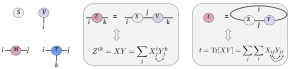
Tensor networks and operations on them are described using an intuitive graphical notation, introduced in Penrose (1971). Figure 2 (left) shows the commonly used notations for a scalar , vector , matrix and a general order- tensor . The number of dimensions of a tensor is captured by the number of edges emanating from the nodes denoted by the edge indices. For instance, the vector is an order- tensor indicated by the edge with index and an order- tensor has three indices depicted by the three edges, and so on.
Tensor notations can also be used to capture operations on higher-order tensors succinctly as shown in Figure 2 (center) where matrix product is depicted, which is also known as tensor contraction. The edge between the tensor nodes and is the dimension subsumed in matrix multiplication resulting in the matrix . More thorough introduction to tensor notations can be found in Bridgeman and Chubb (2017).
2.2 Linear Model in Exponentially High Dimensions
A linear model in a sufficiently high dimensional space can be very powerful (Novikov et al., 2016). In SVMs, this is accomplished by the implicit mapping of the input data into an infinite dimensional space using radial basis function kernels (Hofmann et al., 2008). In this section, we describe the procedure followed in recent tensor network based works, including in ours, to map the input data into an exponentially high dimensional space.
Consider an input vector , which can be obtained by flattening a 2D or 3D image with pixels with intensity values that are normalized in the interval . A commonly used feature map for tensor networks is obtained from the tensor product of pixel-wise feature maps (Stoudenmire and Schwab, 2016):
| (1) |
where the local feature map acting on a pixel is indicated by . The indices run from to where is the dimension of the local feature map. The feature maps are usually simple non-linear functions restricted to have unit norm such that the joint feature map in Eq. (1) also has unit norm. A widely used local feature map with inspired from quantum wave function analysis is (Stoudenmire and Schwab, 2016) is shown in (2), and a simpler local feature map from Efthymiou et al. (2019) in Eq. (3) with similar properties (but non-unit norm):
| (2) | ||||
| (3) |
The joint feature map in Eq. (1) is an order- tensor due to tensor product of the order- local feature maps of dimension in Eq. (2). The joint feature map can be seen as mapping each image to a vector in the dimensional feature space (Stoudenmire and Schwab, 2016). For multi-channel inputs, such as RGB images or other imaging modalities, with input channels the local feature map can be applied to each channel separately such that the resulting space is of dimension (Efthymiou et al., 2019).
Given this high dimensional joint feature map of Eq. (1) for the input data , a linear decision rule for a multi-class classification task can be formulated as:
| (4) | ||||
| (5) |
where are the classes, and the weight tensor is of order-() with the output tensor index .
The tensor notation representation of the linear model of Eq. (5) is shown in Figure 3 (Step 1) where the first column of gray nodes are the individual pixel feature maps of order- with feature dimension . The local feature maps are connected to the order-() weight tensor along edges with one edge for output of dimension marked with index .
The order-(+1) weight tensor results in a total of weight elements. Even for a relatively small gray scale image, say of size , the total number of weight elements in can be massive: which is exponentially more than the number of atoms in the universe555https://en.wikipedia.org/wiki/Observable_universe! The lift in quantum physics is sometimes seen as a convenient illusion (Poulin et al., 2011; Orús, 2014) as the most interesting behavior of systems can be captured with fewer degrees of freedom in this high dimensional space. This is analogous to using fewer than input feature dimensions after dimensionality reduction operations. In the next section we will see how tensor networks can access useful sub-spaces represented by such high dimensional tensors, with parameters that grow linearly with instead of growing exponentially with .
2.3 Matrix Product State (MPS)
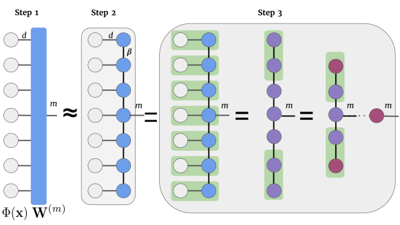
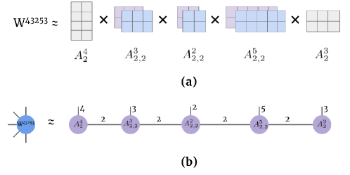
Consider two vectors, and with indices and respectively. The tensor product 666Note that the tensor product of two order-1 tensors is the same as the vector outer product. of these two vectors yields an order- tensor or a matrix . The matrix product state (MPS) (Perez-Garcia et al., 2006) is a type of tensor network that expands on this notion of tensor products allowing the factorization of an order- tensor (with edges) into a chain of lower-order tensors. Specifically, the MPS tensor network can factorise an order- tensor with a chain of order- (with three edges) except on the borders where they are of order-, as shown in Figure 3 (Step 2). Consider a tensor of order- with indices , using MPS it can be approximated using lower-order tensors as
| (6) |
where are the lower-order tensors. The subscript indices are virtual indices that are contracted and are of dimension referred as the bond dimension. The components of these intermediate lower-order tensors form the tunable parameters of the MPS approximation. Note that any dimensional tensor can be represented exactly using an MPS tensor network if . In most applications, however, is fixed to a small value or allowed to adapt dynamically when the MPS tensor network is used to approximate higher-order tensors (Perez-Garcia et al., 2006; Miller, 2019).
One of the drawbacks of using MPS tensor networks is that they operate along one dimension (as a chain). This is the primary reason that two dimensional image data has to be first flattened to a vector when working with tensor networks such as the MPS. Tensor networks that can work on arbitrary graphs, which might be more suitable for image data like the projected entangled pair states (PEPS) (Verstraete and Cirac, 2004), are not as well understood and do not yet have efficient algorithms like the MPS.
Dot product with MPS: The decision function in Eq. (5) comprising the dot product of the order-(+1) weight tensor and the joint feature map in Eq. (1) can be efficiently computed using the MPS approximation in Eq. (6), depicted in Figure 3 (Step 2). The order in which tensor contractions are performed can yield a computationally efficient algorithm. The original MPS algorithm (Perez-Garcia et al., 2006) starts from one of the ends, contracts a pair of tensors to obtain a new tensor which is then contracted with the next tensor and this process is repeated until the output tensor is reached. The cost of this algorithm scales with {} when compared to the cost without the MPS approximation which scales with . In this work, we use the MPS implementation in Miller (2019) which performs parallel contraction of the horizontal edges and then proceeds to contract them vertically as depicted in Figure 3 (Step 3). The MPS approximation also reduces the number of tunable parameters by an exponential factor, from {} to {}.
3 Methods
The primary contribution in this work is a tensor network based image classification model that can handle high resolution images of both two and three spatial dimensions. Several recent tensor network models for supervised image classification tasks operate on small planar images and flatten them into vectors with different raveling strategies at the expense of global image structure (Stoudenmire and Schwab, 2016; Han et al., 2018; Efthymiou et al., 2019). In contrast to these methods, we only flatten small regions of the images which can be assumed to be locally orderless (Koenderink and Van Doorn, 1999) and obtain expressive representations of local image regions using tensor contractions in high dimensional spaces. We process these locally orderless image regions in a hierarchical fashion using layers of MPS blocks in the final model, which we call the locally orderless tensor network (LoTeNet), shown in Figure 6. We next describe the proposed LoTeNet model in detail.
3.1 Squeeze operation
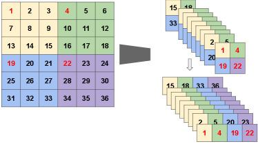
The proposed LoTeNet model operates on small image regions and aggregates them with MPS operations at multiple levels. These small image patches at each level are created using the squeeze operation in two steps, as illustrated in Figure 5 for an order- tensor i.e an image with two spatial dimensions.
The input images are converted into vectors with inflated feature dimensions by applying kernels of stride along each of the spatial dimensions. Consider an input image with spatial dimensions (height:H, width:V, depth:D), pixels and channels as feature dimension: . In the first step, input image is reshaped into smaller patches controlled by the stride : such that the feature dimension increases to . The stride of the kernel decides the extent of reduction in spatial dimensions and the corresponding increase in feature dimension of the squeezed image.
In the second step, the reshaped image patches with inflated feature dimensions are flattened from order- tensors to order- tensors, resulting in with . This flattening operation provides spatial information in the feature dimension to LoTeNet, thus retaining additional image level structure when compared to flattening the entire image into a single vector with channels (Efthymiou et al., 2019). Further, the increase in the feature dimension makes the tensor network more expressive as it increases the dimensionality of the feature space (Stoudenmire and Schwab, 2016).
The transformations in dimensions due to the squeeze operation parameterised by the stride , , are summarised below:
| (7) |
The squeeze operation can also be treated as a local feature map due to the increase in feature dimensions, similar to the more formal pixel level feature maps mentioned in Eq. (2) and Eq. (3), operating on image patches instead of individual pixels. Finally note that the squeeze kernel stride can be different at each level of the model denoted .
In the current formulation, the images are assumed to be rectangular in each plane. As the main purpose of the squeeze operation is to increase the feature dimensions by flattening small local neighbourhoods, this can be achieved by reshaping any small, non-square region of the image into a vector of fixed feature dimension. The simplest strategy to work with non-square (circular images for instance) would be to pad the regions around the borders to make them rectangular. Another approach could be to partition non-square images into cells using Voronoi tesselations (Du et al., 1999) and squeezing these cells into vectors.
3.2 Locally orderless tensor network (LoTeNet)
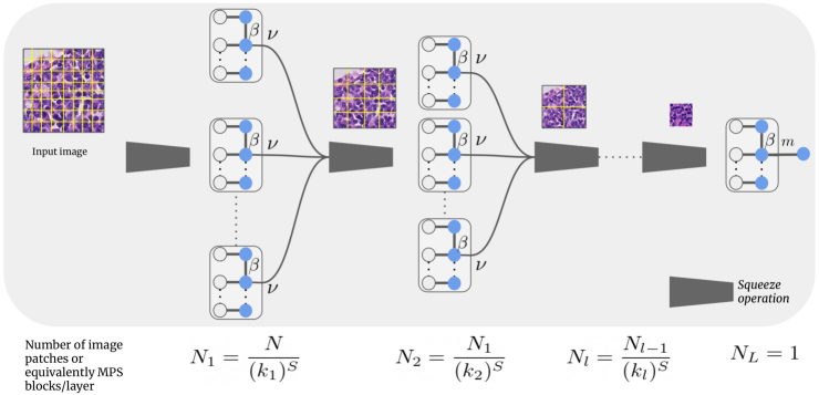
An overview of the proposed LoTeNet model is shown in Figure 6 for an image with two spatial dimensions i.e with . The number of squeezed vectors and the corresponding MPS blocks at each layer of the proposed model are also indicated in Figure 6.
The LoTeNet model comprises of layers of MPS blocks interleaved with squeeze operations without any non-linear components. The input to the first layer in Figure 6 is the full resolution input image with pixels, shown with grids marking the patches which are then squeezed to obtain vectors with . Each of these squeezed patches are input into MPS blocks which contract the vectors to output a vector with dimension . MPS blocks operating on squeezed image patches can be interpreted as summarising them with a vector of size using a linear model in a higher dimensional feature space. In LoTeNet, we set to be the same as the MPS bond dimension , so that there is only a single hyperparameter to be tuned.
The output vectors from all MPS blocks at a given layer are reshaped back into the dimensional image space. However, due to the MPS contractions, these intermediate image space representations will be of lower resolution as indicated by the smaller image with fewer patches in Figure 6. This is analogous to obtaining an average pooled version of the intermediate feature maps in traditional CNNs. The intermediate images of lower resolution formed at layer are further squeezed and contracted in the subsequent layers of the model. This process is continued for layers and the final MPS block acting as layer contracts the output vector from layer to predict the decisions in Eq. (5). The weights of all the MPS blocks in each of the layers are the model parameters which are tuned in a supervised setting as described next.
3.3 Model Optimization
We view the sequence of MPS contractions in successive layers of our model as forward propagation and rely on automatic differentiation to compute the backward computation graph (Efthymiou et al., 2019). Torch MPS package (Miller, 2019) is used to implement MPS blocks and trained in PyTorch (Paszke et al., 2019) to learn the model parameters from training data in an end-to-end fashion. These parameters are analogous to the weights of neural network layers and can be updated in a similar iterative manner by backpropagating a relevant error signal computed between the model predictions and the training labels.
We minimize the cross-entropy loss between the true label for each image and the predicted label in the training set :
| (8) |
where is the softmax operation used to obtain normalized scores that can be interpreted as the predicted class probabilities. For binary classes, the loss in Eq. (8) reduces to the binary cross entropy and output dimension can be used with the sigmoid non-linearity to obtain probabilistic predictions in .
4 Related work
Key ideas in the proposed locally orderless tensor network are related to several existing methods in the literature. The closest of them is the tensor network model in Efthymiou et al. (2019) which in turn was based on the work in Stoudenmire and Schwab (2016). The primary difference of LoTeNet compared to Efthymiou et al. (2019) is in its ability to handle high resolution 2D/3D images without losing spatial correlation between pixels. This capability is incorporated with strategies from image analysis such as the interpretation of small regions to be orderless (Koenderink and Van Doorn, 1999). Further, the multi-layered approach used in LoTeNet has similarities with the multi-scale analysis of images (Lindeberg, 2007).
The squeeze operation described in Section 3.1 serves dual purposes: to move spatial information into feature dimension and to increase the feature dimension. This is based on similar operations performed in normalizing flow literature to provide additional spatial context via feature dimensions such as in Dinh et al. (2017). The operation of stacking pixels into feature dimension is also similar to the im2col operations used to transform convolution into multiplications for improving efficiency of deep learning operations (Chetlur et al., 2014). Recently, in Blendowski and Heinrich (2020), the im2col operation was also used as a preprocessing step with differentiable decision trees such as random ferns (Ozuysal et al., 2009). The squeeze operation can also been as the inverse of the pixel shuffle operation introduced in Shi et al. (2016) where the feature maps are interleaved into spatial dimension to perform sub-pixel convolution.
5 Data and Experiments
5.1 Data
We report experiments on three public datasets for the task of binary classification from 2D histopathology slides, 2D thoracic computed tomography (CT) and 3D T1-weighted MRI scans.
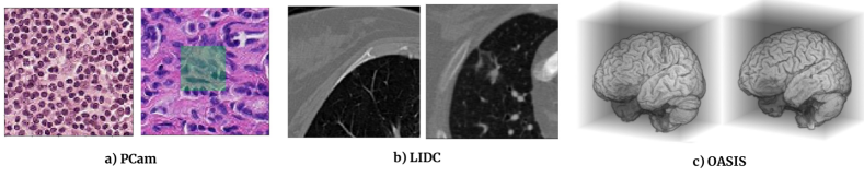
PCam Dataset: The PatchCamelyon (PCam) dataset is a binary histopathology image classification dataset introduced in Veeling et al. (2018). Image patches of size px are extracted from the Camelyon16 Challenge dataset (Bejnordi et al., 2017) with positive label indicating the presence of at least one pixel of tumour tissue in the central px region and a negative label indicating absence of tumour, as shown in Figure 7(a). In this work, a modified PCam dataset from the Kaggle challenge777https://www.kaggle.com/c/histopathologic-cancer-detection is used that removes duplicate image patches included in the original dataset. This dataset consists of about patches for training and an independent test set of about patches is provided for evaluating the models. Data augmentation is performed during training with probability comprising of rotation, horizontal and vertical flips.
LIDC Dataset: The LIDC-IDRI datatset comprises of 1018 thoracic CT images with lesions annotated by four radiologists (Armato III et al., 2004). We use the px 2D slices from Knegt (2018) (shown in Figure 7 (b)) yielding a total of patches. The segmentation masks from the four raters are transformed to binary labels indicating the presence (if two or more radiologists marked a tumour) or absence of tumours (if less than two raters marked tumours). These binary labels capture a majority voting among the radiologists. The dataset is split into splits for training, validation and a hold-out test set.
OASIS Dataset: The OASIS dataset consists of T1-weighted MRI scans of 416 subjects aged between 18 to 96 years (Marcus et al., 2007). The scans are graded with clinical dementia rating (CDR) into four classes: non-demented=0, very mild dementia=0.5, mild dementia=1.0, moderate dementia=2.0. We create an Alzheimer’s disease classification dataset according to Wen et al. (2020) with scans of all subjects above 60 years resulting in a dataset with 155 subjects. Binary labels are extracted from the CDR scores: cognitively normal (CN) if CDR=0 and Alzheimer’s disease (AD) if CDR0, yielding 82:73 split between CN and AD cases. The MRI scans are preprocessed using the extensive pipeline described in Wen et al. (2020) comprising bias field correction, non-linear registration and skull stripping using the ClincaDL package888https://clinicadl.readthedocs.io/en/latest/. After preprocessing we obtain volumes of size 128x128x128 voxels (Figure 7-c).
5.2 Experiments and Results
5.2.1 Implementation
The model is implemented in PyTorch (Paszke et al., 2019) based on the Torch MPS package (Miller, 2019). The architecture of LoTeNet model is kept fixed across all the datasets. The proposed LoTeNet model is evaluated with layers, squeeze kernel of size except for the input layer where in order to reduce the number of MPS blocks in the first layer. The most critical hyperparameter of LoTeNet is its bond dimension ; it was set to obtained from the range based on the performance on the PCam validation set. We set the virtual dimension to be the same as the bond dimension. Note that increasing the depth in LoTeNet does not translate to obtaining more complex decisions (like in neural networks) as LoTeNet is a linear model. Number of layers are controlled by the kernel stride and primarily result in reduced computation cost (Selvan et al., 2020). Finally, to keep the number of tunable hyperparameters lower, we also do not optimize and jointly which would yield a model similar to an adaptive MPS (Stoudenmire and Schwab, 2016; Miller, 2019)
We use the Adam optimizer (Kingma and Ba, 2014) with a learning rate of . We use a batch size of for experiments on the PCam and LIDC datasets, and a batch size of for the OASIS dataset. We incorporate batch normalisation (Ioffe and Szegedy, 2015) after each layer in all the models and we observed this resulted in faster and more robust convergence. All models were assumed to have converged if there was no improvement in validation accuracy over consecutive epochs and the model with the best validation performance was used to predict on the test set. All experiments were run on a single Tesla K80 GPU with 12 GB memory. The development and training of all models (including baselines) in this work is estimated to produce 14.1 kg of CO2eq, equivalent to 120.1 km travelled by car as measured by Carbontracker 999https://github.com/lfwa/carbontracker/ (Anthony et al., 2020).
5.2.2 Experiments on 2D data
| PCam Models | GPU(GB) | AUC |
|---|---|---|
| Rotation Eq-CNN | ||
| Densenet | ||
| LoTeNet (ours) | ||
| Tensor Net-X () |
| LIDC Models | GPU(GB) | AUC |
|---|---|---|
| LoTeNet (ours) | ||
| Tensor Net-X ( | ||
| Densenet | ||
| Tensor Net-X ( |
PCam models: Performance of the LoTeNet model is compared to the rotation equivariant CNNs in (Veeling et al., 2018) which is also state-of-the-art for the PCam dataset. Additionally, we compare to the single layer MPS model with local feature map of the form in Eq. (3) with from Efthymiou et al. (2019) reported here as Tensor Net-X and to Densenet (Huang et al., 2017) with layers and a growth rate of . We compare the binary classification performance of the models using the area under the ROC curve (AUC) as it is not sensitive to arbitrary decision thresholds. The performance metrics are shown in Table 1 (left) along with the maximum GPU memory utilisation for each of the models. We observe the AUC on the test set attained by LoTeNet model () is comparable to the Rotation Eq. CNN () and Densenet models () on the PCam dataset with a drastic reduction in the maximum GPU memory utilisation; a mere 0.8 GB when compared to upto 11 GB for the Rotation Eq.CNN 101010In Veeling et al. (2018) the authors used 4x12GB GPUs which was confirmed to R.Selvan by B.Veeling. and 10.5 GB for Densenet. We also notice a considerable improvement when compared to Tensor Net-X in the attained AUC (0.908).
LIDC models: Similar to the PCam dataset, performance of LoTeNet model is compared using AUC and maximum GPU memory utilisation, and are reported in Table 1 (right). We compare to Densenet and Tensor Net-X with two bond dimensions () to highlight the influence of the bond dimension. LoTeNet model fares better than the compared models with an AUC of whereas the Densenet model achieves and Tensor Net-X achieves () and (). The GPU memory utlisation follows a similar trend as with the PCam models with LoTeNet requiring only GB.
5.2.3 Experiments on 3D data
LoTeNet used in the 3D experiments is identical to the one used in 2D experiments except for the local feature map. For the 3D experiments, we do not apply the local feature map in Eq. (2) but instead rely on the increase in feature dimension due to the squeeze operation in Eq. (7). This reduces the number of parameters of the LoTeNet model and the risk of overfitting to the limited data in the OASIS dataset.
The experimental set-up closely follows from Wen et al. (2020) and we use 5-fold cross validation to report the balanced accuracy on each of the test folds. Balanced accuracy (BA) is binary accuracy normalised by the class skew and helps when the classes are imbalanced. We reimplemented the subject-level 3D CNN used in Wen et al. (2020) as one of the compared methods. The subject-level CNN comprises 5 layers of 3D CNN with an initial feature map of , max pooling and rectified linear units (ReLU) with doubling of feature maps after each layer, and an additional three linear layers with ReLUs to output the final predictions. We also report two other baseline models based on 3D CNN and a multi-layered perceptron (MLP) model. The CNN baseline model is similar to the subject-level CNN but has an initial feature map size of . The MLP baseline has four layers to match the LoTeNet model, and ReLU non-linear activation function.
Table 2 summarises the performance of LoTeNet along with the compared methods for two types of inputs. As LoTeNet is agnostic to the dimensionality of the input image due to the squeeze operations, we demonstrate the performance on volume data (3D) and also on 19,840 slices extracted along the z-axis (2D) from the volume data. For the 2D experiments we ensure there is no data leakage by creating folds at subject level. The balanced accuracy across five test folds are shown and we see a clear improvement () for the 3D case compared to subject-level CNN model (). LoTeNet model has a lower score in the 2D case, indicating the model is able to extract more global information from the volume data than from 2D slices. Additionally, we report the number of parameters, maximum GPU utilisation and time per training epoch for all the methods. To show the influence of the number of parameters, we compare to a large MLP baseline model with 78M parameters and observe this increase does not necessarily improve the baseline model’s performance.
| OASIS Models | Input | # Param. | GPU (GB) | t (s) | Average BA |
| LoTeNet (ours) | 3D | 52M | 45.3 | ||
| Subject-level CNN | 3D | 1M | 8.7 | ||
| CNN Baseline | 3D | 6.4M | 12.8 | ||
| MLP Baseline | 3D | 78M | 4.1 | ||
| Densenet | 2D | 0.2M | 80.1 | ||
| LoTeNet (ours) | 2D | 0.4M | 81.3 |
6 Discussion
In this section, we focus on discussing high level trends observed with experiments reported in Section 5.2, conceptual connections to other methods, and point out possible directions for future work.
6.1 Comparison with tensor network models
The proposed LoTeNet model is related to the tensor network models used for supervised learning tasks, such as the ones in Stoudenmire and Schwab (2016); Efthymiou et al. (2019). In Stoudenmire and Schwab (2016), the parameters of the tensor network are learned from data using density matrix renormalization group (DMRG) algorithm (McCulloch, 2007), whereas in LoTeNet we use automatic differentiation based on the implementation in Miller (2019) similar to Efthymiou et al. (2019) to optimise the parameters of the model in Eq. (6).
The proposed LoTeNet model also improves upon the computation cost of approximating linear decisions compared to other tensor network models such as in Efthymiou et al. (2019). Consider the computation cost of approximating the linear decision in Eq. (5) for an input image with pixels of features with a bond dimension . For the tensor network in Efthymiou et al. (2019) it is . For LoTeNet, the computation cost reduces exponentially with the number of layers used: . The spatial resolution of the input image is reduced with successive layers in LoTeNet (Figure 6) captured as the term in the denominator. The cost of performing MPS operations on patches of size in layers is the additional term in the numerator. However, for and , the exponential reduction in computation cost with can translate into considerable computational advantage when processing high resolution medical images. Further, the computation cost of LoTeNet can be reduced without noticeable degradation in performance by sharing MPS in each layer across all patches (Selvan et al., 2020).
6.2 On Performance
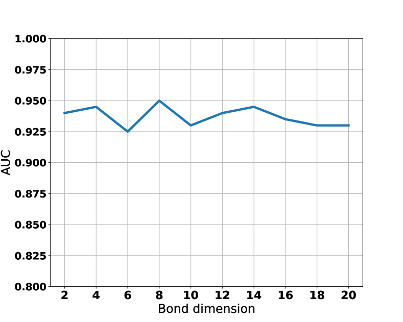
The performance of LoTeNet across the three datasets is on par with, or superior, to the other methods as reported in Tables 1 and 2. This robustness across tasks is remarkable because the LoTeNet architecture is fixed across the tasks. This behaviour could be attributed to the single model hyperparameter – bond dimension, – which is fixed () across all experiments. Recollect that the bond dimension controls the quality of MPS approximations of the corresponding operations in high dimensional spaces as described in Section 2.3. Consistent with the reporting in earlier works (Efthymiou et al., 2019), we also find that the value of after a specific value does not affect the model’s performance. This is illustrated in Figure 8, where we show the sensitivity of the validation set performance on LIDC dataset for different bond dimensions. This is a desirable feature as the models can be expected to yield comparable performance when applied to different datasets without entailing dataset specific cost of elaborate architecture search. Additionally, this robustness could also be attributed to more efficient computation of massive number of parameters in LoTeNet resulting in generalised decision rules, as reported in Table 2 where we notice that the number of parameters in LoTeNet are higher than other methods (except MLP baseline).
In Tables 1 and 2, we report the GPU memory requirement for each of the models. LoTeNet requires only a fraction of the GPU memory utilised by the corresponding baseline methods, including the Densenet (Huang et al., 2017) or Rotation Eq-CNN models (Veeling et al., 2018). One reason for this drastic reduction in GPU memory utilisation is because tensor networks do not maintain massive intermediate feature maps. This behaviour is similar to feedforward neural networks and unlike CNNs which use a large chunk of GPU memory mainly to store intermediate feature maps (Rhu et al., 2016). Further, as LoTeNet is based on contracting input data into smaller tensors in a hierarchical manner the memory consumption with successive contracted layers does not increase. This can be an important feature in medical imaging applications as larger images and larger batch sizes can be processed without compromising the quality of the learned decision rules.
6.3 Choice of local feature maps
The local feature maps in Equations (2) and (3) are simple transformations which have been used in the tensor network literature (Stoudenmire and Schwab, 2016; Efthymiou et al., 2019). More recently, other intensity based local feature maps such as wavelet transforms have been attempted for 1D signal classification in Reyes and Stoudenmire (2020). While we use the local map in Equation (2) for 2D data and squeeze operation based local map for 3D data, experiments on other possible local feature maps were also performed. For instance, we experimented with jet based feature maps (Larsen et al., 2012) that compute spatial gradients at multiple scales, and also an MLP based local feature map acting on individual pixels. Both these local feature maps did not yield any considerable performance improvement and to adhere to existing tensor network literature we used the simple sinusoidal feature maps which also do not have additional hyperparameters.
6.4 Comparison with Neural Networks
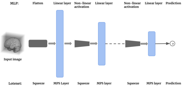
Feed-forward neural networks: The class of tensor network models adapted for machine learning tasks (Stoudenmire and Schwab, 2016; Efthymiou et al., 2019) are conceptually most similar to feed-forward neural networks such as the MLP, as both classes of models operate on vector inputs (see Figure 9). The difference, however, arises in the type of decision boundaries optimised by each class of model as illustrated in Figure 1. MLP based feed-forward networks obtain non-linear decision boundaries using several layers of neurons and non-linear activation functions (such as sigmoid, ReLU etc.). Tensor network models, including the proposed model, optimise linear decision boundaries in exponentially high dimensional spaces without using any non-linear activation functions.
Convolutional neural networks: LoTeNet uses MPS blocks on image patches and aggregates these tensor representations in a hierarchical manner to learn the decision rule. While this could appear similar to the use of strided convolution kernels in CNNs, it is indeed closer to feed-forward neural networks. The use of an MPS block per patch perhaps can be interpreted as a form of strided convolution but only in how the local operation is performed on each patch. The primary difference is in the weight sharing; the weights of MPS blocks are not shared across the image. Each image region has an MPS block acting on it. This is indicated in Figure 6, where we report the number of MPS blocks used per layer.
6.5 Limitations and Future Work
The computation time reported in Table 2 shows it to be higher for LoTeNet (s) compared to the CNN (s) or MLP (s) baselines as efficient implementations of tensor contractions are not natively supported in frameworks such as PyTorch. There are ongoing efforts to further improve efficient implementations which can accelerate tensor network operations (Fishman et al., 2020; Novikov et al., 2020). Considering that LoTeNet usually converges between 10-20 epochs, the increase in computation time with the current implementation is not substantial as the model can be trained even on 3D data easily under an hour.
One possible drawback of having a single hyperparameter controlling the MPS approximations is the lack of granular control of the model capacity. In the 2D OASIS experiments (Table 2), we further investigated the lower average balanced accuracy score by trying out different values. This experiment revealed that LoTeNet was either under-fitting () or over-fitting () to the training set. This could be attributed to the fact that the number of parameters grow quadratically with and these discrete jumps make it harder to obtain models of optimal capacity for some tasks.
Another concern with tensor network based models is their tendency to be over parameterised as the number of parameters scale as {}. The linear dependency on the number of pixels, , for volumetric data results in a model with massive number of parameters at the outset which is further aggravated by the quadratic dependency on . While in our experiments, this has not had an adverse effect on the performance, we have observed the model is capable of over-fitting on small training data quite easily. This can be a concern when dealing with datasets with few samples.
One way of handling these problems would be to introduce weight-sharing between MPS blocks at each layer so that the number of parameters can be reduced and controlled better. A possible future work is to investigate the effect of sharing MPS blocks per layer and study if equivariance to translation can be induced in tensor network based models (Cohen and Welling, 2016).
Finally, the issue of extending LoTeNet type models beyond classification or regression tasks to more diverse medical imaging tasks such as segmentation and registration are open research questions waiting to be explored further. Early work on using tensor networks for 2D segmentation tasks was recently reported in Selvan et al. (2021).
7 Conclusion
We have presented a tensor network model for classification of 2D and 3D medical images, of higher spatial resolutions. Using LoTeNet we have shown that aggregating MPS approximations on small image regions in a hierarchical manner retains global structure of the image data. With experiments on three datasets we have shown such models can yield competitive performance on a variety of classification tasks. We have measured the GPU memory requirement of the proposed model and shown it to be a fraction of the memory utilisation of state-of-the-art CNN based models when trained to attain comparable performance. Finally, we have demonstrated that a single model architecture with (tuned on one of the datasets) can perform well on other datasets also, which can be an appealing feature as it reduces dataset specific architecture search.
Acknowledgments
Data used in this work were provided in part by OASIS: Cross-Sectional: Principal Investigators: D. Marcus, R, Buckner, J, Csernansky J. Morris; P50 AG05681, P01 AG03991, P01 AG026276, R01 AG021910, P20 MH071616, U24 RR021382. We thank Eric Kim for permitting us to modify and use Figure 1. The authors also thank all reviewers and editors for their insightful feedback.
Ethical Standards
The work follows appropriate ethical standards in conducting research and writing the manuscript. All data used in this project are from open repositories.
Conflicts of Interest
We declare we do not have conflicts of interest.
References
- Anthony et al. [2020] Lasse F. Wolff Anthony, Benjamin Kanding, and Raghavendra Selvan. Carbontracker: Tracking and predicting the carbon footprint of training deep learning models. ICML Workshop on Challenges in Deploying and monitoring Machine Learning Systems, July 2020. arXiv:2007.03051.
- Armato III et al. [2004] Samuel G Armato III, Geoffrey McLennan, Michael F McNitt-Gray, Charles R Meyer, David Yankelevitz, Denise R Aberle, Claudia I Henschke, Eric A Hoffman, Ella A Kazerooni, Heber MacMahon, et al. Lung image database consortium: developing a resource for the medical imaging research community. Radiology, 232(3):739–748, 2004.
- Bejnordi et al. [2017] Babak Ehteshami Bejnordi, Mitko Veta, Paul Johannes Van Diest, Bram Van Ginneken, Nico Karssemeijer, Geert Litjens, Jeroen AWM Van Der Laak, Meyke Hermsen, Quirine F Manson, Maschenka Balkenhol, et al. Diagnostic assessment of deep learning algorithms for detection of lymph node metastases in women with breast cancer. Jama, 318(22):2199–2210, 2017.
- Blendowski and Heinrich [2020] Max Blendowski and Mattias P. Heinrich. Learning to map between ferns with differentiable binary embedding networks. In Medical Imaging with Deep Learning, 2020. URL https://openreview.net/forum?id=sdSOFa3Y09.
- Bordes et al. [2005] Antoine Bordes, Seyda Ertekin, Jason Weston, and Léon Bottou. Fast kernel classifiers with online and active learning. Journal of Machine Learning Research, 6(Sep):1579–1619, 2005.
- Boser et al. [1992] Bernhard E Boser, Isabelle M Guyon, and Vladimir N Vapnik. A training algorithm for optimal margin classifiers. In Proceedings of the fifth annual workshop on Computational learning theory, pages 144–152, 1992.
- Bridgeman and Chubb [2017] Jacob C Bridgeman and Christopher T Chubb. Hand-waving and interpretive dance: an introductory course on tensor networks. Journal of Physics A: Mathematical and Theoretical, 50(22):223001, 2017.
- Burges [1998] Christopher JC Burges. A tutorial on support vector machines for pattern recognition. Data mining and knowledge discovery, 2(2):121–167, 1998.
- Cheng et al. [2019] Song Cheng, Lei Wang, Tao Xiang, and Pan Zhang. Tree tensor networks for generative modeling. Physical Review B, 99(15):155131, 2019.
- Chetlur et al. [2014] Sharan Chetlur, Cliff Woolley, Philippe Vandermersch, Jonathan Cohen, John Tran, Bryan Catanzaro, and Evan Shelhamer. cudnn: Efficient primitives for deep learning. arXiv preprint arXiv:1410.0759, 2014.
- Cichocki et al. [2016] Andrzej Cichocki, Namgil Lee, Ivan Oseledets, Anh-Huy Phan, Qibin Zhao, Danilo P Mandic, et al. Tensor networks for dimensionality reduction and large-scale optimization: Part 1 low-rank tensor decompositions. Foundations and Trends® in Machine Learning, 9(4-5):249–429, 2016.
- Cohen et al. [2016] Nadav Cohen, Or Sharir, and Amnon Shashua. On the expressive power of deep learning: A tensor analysis. In Conference on Learning Theory, pages 698–728, 2016.
- Cohen and Welling [2016] Taco Cohen and Max Welling. Group equivariant convolutional networks. In International conference on machine learning, pages 2990–2999, 2016.
- Cortes and Vapnik [1995] Corinna Cortes and Vladimir Vapnik. Support-vector networks. Machine learning, 20(3):273–297, 1995.
- Dinh et al. [2017] Laurent Dinh, Jascha Sohl-Dickstein, and Samy Bengio. Density estimation using Real NVP. In International Conference on Learning Representation, 2017.
- Du et al. [1999] Qiang Du, Vance Faber, and Max Gunzburger. Centroidal voronoi tessellations: Applications and algorithms. SIAM review, 41(4):637–676, 1999.
- Efthymiou et al. [2019] Stavros Efthymiou, Jack Hidary, and Stefan Leichenauer. Tensornetwork for Machine Learning. arXiv preprint arXiv:1906.06329, 2019.
- Fannes et al. [1992] Mark Fannes, Bruno Nachtergaele, and Reinhard F Werner. Finitely correlated states on quantum spin chains. Communications in mathematical physics, 144(3):443–490, 1992.
- Fishman et al. [2020] Matthew Fishman, Steven R White, and E Miles Stoudenmire. The itensor software library for tensor network calculations. arXiv preprint arXiv:2007.14822, 2020.
- Glasser et al. [2019] Ivan Glasser, Ryan Sweke, Nicola Pancotti, Jens Eisert, and Ignacio Cirac. Expressive power of tensor-network factorizations for probabilistic modeling. In Advances in Neural Information Processing Systems, pages 1496–1508, 2019.
- Han et al. [2018] Zhao-Yu Han, Jun Wang, Heng Fan, Lei Wang, and Pan Zhang. Unsupervised generative modeling using matrix product states. Physical Review X, 8(3):031012, 2018.
- Hofmann et al. [2008] Thomas Hofmann, Bernhard Schölkopf, and Alexander J Smola. Kernel methods in machine learning. The annals of statistics, pages 1171–1220, 2008.
- Huang et al. [2017] Gao Huang, Zhuang Liu, Laurens Van Der Maaten, and Kilian Q Weinberger. Densely connected convolutional networks. In Proceedings of the IEEE conference on computer vision and pattern recognition, pages 4700–4708, 2017.
- Ioffe and Szegedy [2015] Sergey Ioffe and Christian Szegedy. Batch normalization: Accelerating deep network training by reducing internal covariate shift. arXiv preprint arXiv:1502.03167, 2015.
- Kingma and Ba [2014] Diederik P Kingma and Jimmy Ba. Adam: A method for stochastic optimization. arXiv preprint arXiv:1412.6980, 2014.
- Klus and Gelß [2019] Stefan Klus and Patrick Gelß. Tensor-based algorithms for image classification. Algorithms, 12(11):240, 2019.
- Knegt [2018] Stefan Knegt. A Probabilistic U-Net for segmentation of ambiguous images implemented in PyTorch. https://github.com/stefanknegt/Probabilistic-Unet-Pytorch, 2018.
- Koenderink and Van Doorn [1999] Jan J Koenderink and Andrea J Van Doorn. The structure of locally orderless images. International Journal of Computer Vision, 31(2-3):159–168, 1999.
- Larsen et al. [2012] Anders Boesen Lindbo Larsen, Sune Darkner, Anders Lindbjerg Dahl, and Kim Steenstrup Pedersen. Jet-based local image descriptors. In European Conference on Computer Vision, pages 638–650. Springer, 2012.
- Lindeberg [2007] Tony Lindeberg. Scale-space. Wiley Encyclopedia of Computer Science and Engineering, pages 2495–2504, 2007.
- Litjens et al. [2017] Geert Litjens, Thijs Kooi, Babak Ehteshami Bejnordi, Arnaud Arindra Adiyoso Setio, Francesco Ciompi, Mohsen Ghafoorian, Jeroen Awm Van Der Laak, Bram Van Ginneken, and Clara I Sánchez. A survey on deep learning in medical image analysis. Medical image analysis, 42:60–88, 2017.
- Liu et al. [2017] Peng Liu, Kim-Kwang Raymond Choo, Lizhe Wang, and Fang Huang. Svm or deep learning? a comparative study on remote sensing image classification. Soft Computing, 21(23):7053–7065, 2017.
- Marcus et al. [2007] Daniel S Marcus, Tracy H Wang, Jamie Parker, John G Csernansky, John C Morris, and Randy L Buckner. Open access series of imaging studies (oasis): cross-sectional mri data in young, middle aged, nondemented, and demented older adults. Journal of cognitive neuroscience, 19(9):1498–1507, 2007.
- McCulloch [2007] Ian P McCulloch. From density-matrix renormalization group to matrix product states. Journal of Statistical Mechanics: Theory and Experiment, 2007(10):P10014, 2007.
- Miller [2019] Jacob Miller. Torchmps. https://github.com/jemisjoky/torchmps, 2019.
- Novikov et al. [2016] Alexander Novikov, Mikhail Trofimov, and Ivan Oseledets. Exponential machines. arXiv preprint arXiv:1605.03795, 2016.
- Novikov et al. [2020] Alexander Novikov, Pavel Izmailov, Valentin Khrulkov, Michael Figurnov, and Ivan V Oseledets. Tensor train decomposition on tensorflow (t3f). Journal of Machine Learning Research, 21(30):1–7, 2020.
- Orús [2014] Román Orús. A practical introduction to tensor networks: Matrix product states and projected entangled pair states. Annals of Physics, 349:117–158, 2014.
- Oseledets [2011] Ivan V Oseledets. Tensor-train decomposition. SIAM Journal on Scientific Computing, 33(5):2295–2317, 2011.
- Ozuysal et al. [2009] Mustafa Ozuysal, Michael Calonder, Vincent Lepetit, and Pascal Fua. Fast keypoint recognition using random ferns. IEEE transactions on pattern analysis and machine intelligence, 32(3):448–461, 2009.
- Paszke et al. [2019] Adam Paszke, Sam Gross, Francisco Massa, Adam Lerer, James Bradbury, Gregory Chanan, Trevor Killeen, Zeming Lin, Natalia Gimelshein, Luca Antiga, et al. Pytorch: An imperative style, high-performance deep learning library. In Advances in Neural Information Processing Systems, pages 8024–8035, 2019.
- Penrose [1971] Roger Penrose. Applications of negative dimensional tensors. Combinatorial mathematics and its applications, 1:221–244, 1971.
- Perez-Garcia et al. [2006] David Perez-Garcia, Frank Verstraete, Michael M Wolf, and J Ignacio Cirac. Matrix product state representations. arXiv preprint quant-ph/0608197, 2006.
- Poulin et al. [2011] David Poulin, Angie Qarry, Rolando Somma, and Frank Verstraete. Quantum simulation of time-dependent hamiltonians and the convenient illusion of hilbert space. Physical review letters, 106(17), 2011.
- Reyes and Stoudenmire [2020] Justin Reyes and Miles Stoudenmire. A multi-scale tensor network architecture for classification and regression. arXiv preprint arXiv:2001.08286, 2020.
- Rhu et al. [2016] Minsoo Rhu, Natalia Gimelshein, Jason Clemons, Arslan Zulfiqar, and Stephen W Keckler. vdnn: Virtualized deep neural networks for scalable, memory-efficient neural network design. In 2016 49th Annual IEEE/ACM International Symposium on Microarchitecture (MICRO), pages 1–13. IEEE, 2016.
- Sagan [2012] Hans Sagan. Space-filling curves. Springer Science & Business Media, 2012.
- Selvan and Dam [2020] Raghavendra Selvan and Erik B Dam. Tensor networks for medical image classification. In International Conference on Medical Imaging with Deep Learning – Full Paper Track, volume 121 of Proceedings of Machine Learning Research, pages 721–732. PMLR, 06–08 Jul 2020. URL http://proceedings.mlr.press/v121/selvan20a.html.
- Selvan et al. [2020] Raghavendra Selvan, Silas Ørting, and Erik B Dam. Multi-layered tensor networks for image classification. In First NeurIPS Workshop on Quantum Tensor Networks in Machine Learning, 2020.
- Selvan et al. [2021] Raghavendra Selvan, Erik B Dam, and Jens Petersen. Segmenting two-dimensional structures with strided tensor networks. In 27th International Conference on Information Processing in Medical Imaging (IPMI-2021), Bornholm, Denmark., 2021.
- Shi et al. [2016] Wenzhe Shi, Jose Caballero, Ferenc Huszár, Johannes Totz, Andrew P Aitken, Rob Bishop, Daniel Rueckert, and Zehan Wang. Real-time single image and video super-resolution using an efficient sub-pixel convolutional neural network. In Proceedings of the IEEE conference on computer vision and pattern recognition, pages 1874–1883, 2016.
- Shi et al. [2006] Y-Y Shi, L-M Duan, and Guifre Vidal. Classical simulation of quantum many-body systems with a tree tensor network. Physical review a, 74(2):022320, 2006.
- Stoudenmire and Schwab [2016] Edwin Stoudenmire and David J Schwab. Supervised learning with tensor networks. In Advances in Neural Information Processing Systems, pages 4799–4807, 2016.
- Sun et al. [2020] Zheng-Zhi Sun, Cheng Peng, Ding Liu, Shi-Ju Ran, and Gang Su. Generative tensor network classification model for supervised machine learning. Physical Review B, 101(7):075135, 2020.
- Veeling et al. [2018] Bastiaan S Veeling, Jasper Linmans, Jim Winkens, Taco Cohen, and Max Welling. Rotation equivariant CNNs for digital pathology. In International Conference on Medical image computing and computer-assisted intervention, pages 210–218. Springer, 2018.
- Verstraete and Cirac [2004] Frank Verstraete and J Ignacio Cirac. Renormalization algorithms for quantum-many body systems in two and higher dimensions. arXiv preprint cond-mat/0407066, 2004.
- Wen et al. [2020] Junhao Wen, Elina Thibeau-Sutre, Mauricio Diaz-Melo, Jorge Samper-González, Alexandre Routier, Simona Bottani, Didier Dormont, Stanley Durrleman, Ninon Burgos, Olivier Colliot, et al. Convolutional Neural Networks for Classification of Alzheimer’s Disease: Overview and Reproducible Evaluation. Medical Image Analysis, page 101694, 2020.