PathologyGAN: Learning deep representations of cancer tissue

Quiros, Adalberto Claudio; Murray-Smith, Roderick; Yuan, Ke

doi:https://doi.org/10.59275/j.melba.2021-gfgg

1 Introduction

Cancer is a disease with extensive heterogeneity, where malignant cells interact with immune cells, stromal cells, surrounding tissues and blood vessels. Histological images, such as haematoxylin and eosin (H&E) stained tissue microarrays (TMAs) or whole slide images (WSI), are a high-throughput imaging technology used to study such diversity. Despite being ubiquitous in clinical settings, analytical tools of H&E images remain primitive, making these valuable data largely under-explored. Consequently, cellular behaviours and the tumor microenvironment recorded in H&E images remain poorly understood. Increasing our understanding of such microenvironment interaction holds the key for improved diagnosis and treatment of cancer.

Refer to caption — Figure 1: (a): Images ( $224\times 224$ ) from PathologyGAN trained on H&E breast cancer tissue. (b): Real images, Inception-V1 closest neighbor to the generated above in (a). (c): Images ( $224\times 224$ ) from PathologyGAN trained on H&E colorectal cancer tissue. (d) Real images, Inception-V1 closest neighbor to the generated above in (c).

The motivation for our work is to develop methods that could lead to a better understanding of phenotype diversity between/within tumors. We hypothesize that this diversity could be substantial given the highly diverse genomic and transcriptomic landscapes observed in large scale molecular profiling of tumors across multiple cancer types (Campbell et al., 2020). We argue that representation learning with GAN-based models is the most promising to achieve our goal for the two following reasons:

1.
By being able to generate high fidelity images, a GAN could learn the most relevant descriptions of tissue phenotype.
2.
The continuous latent representation learned by GANs could help us quantify differences in tissue architectures free from supervised information.

In this paper, we propose to use Generative Adversarial Networks (GANs) to learn representations of entire tissue architectures and define an interpretable latent space (e.g. colour, texture, spatial features of cancer and normal cells, and their interaction). To this end, we present the following contributions:

1.
We propose PathologyGANs to generate high fidelity cancer tissue images from a structured latent space. The model combines BigGAN (Brock et al., 2019), StyleGAN (Karras et al., 2019) and Relativistic Average Discriminator (Jolicoeur-Martineau, 2019).
2.
We assess the quality of the generated images through two different methods: convolutional Inception-V1 features and prognostic features of the cancer tissue, such as counts and densities of different cell types (Beck et al., 2011; Yuan et al., 2012). Both features are benchmarked with the Fréchet Inception Distance (FID). The results show that the model captures pathologically meaningful representations, and when evaluated by expert pathologists, generated tissue images are not distinct from real tissue images.
3.
We show that our model induces an ordered latent space based on tissue characteristics (e.g. cancer cell density or tissue type), this allows to perform linear vector operations that transfer into high level tissue image changes.

2 Related Works

Deep learning has been widely applied in digital pathology, from these we can differentiate between supervised and unsupervised learning approaches.

Supervised applications range from mitosis and cell detection (Tellez et al., 2018; Xu et al., 2019a; Zhang et al., 2019b), nuclei and tumor segmentation (Qu et al., 2019; Qaiser et al., 2019), histological subtype classification (Coudray et al., 2018; Wei et al., 2019), to survival and prognosis modeling (Katzman et al., 2018; Lee et al., 2018). Recently, there have been developments on relating phenotype to the molecular underpining of tumors, in particular genomic characteristics (Coudray et al., 2018; Schmauch et al., 2020; Woerl et al., 2020; Fu et al., 2020; Coudray and Tsirigos, 2020; Kather et al., 2020), and spatial transcriptomics (Vickovic et al., 2019; He et al., 2020; Bergenstråhle et al., 2020a; Schmauch et al., 2020; Wang et al., 2020; Bergenstråhle et al., 2020b). Furthermore, previous traditional computer vision approaches (Beck et al., 2011; Yuan et al., 2012) already identified correlation between phenotype patterns and patient survival. These works highlight the importance and opportunities that building tissue phenotype representations bring, providing insight into survival or genomic information purely from tissue images such as TMA or WSIs.

Nevertheless, these methods require data labeling which is usually costly in time and effort, this is particularly the case for sequencing derived molecular labels. In addition, deep learning approaches have a lack of interpretability, which is also a major limiting factor in making a real impact in clinical practice.

Unsupervised learning applications mostly focus on nuclei (Xu et al., 2016; Mahmood et al., 2018), tissue (de Bel et al., 2018), or region-of-interest segmentation (Gadermayr et al., 2018, 2019), besides stain transformation (Rana et al., 2018; Xu et al., 2019b) and normalization (Zanjani et al., 2018). Within unsupervised learning, generative models have been briefly used for tissue generation (Levine et al., 2020), however this model lacks of representation learning properties. On the other hand, there has been some initial work on building cell and nuclei representations with models such as InfoGAN (Hu et al., 2019) and Sparse Auto-Encoders (Hou et al., 2019), although these models focus either on small sections of images or cells instead of larger tiles of tissue.

Building phenotype representations based on tissue architecture and cellular attributes remains a field to be further explored. Generative models offer the ability to create tissue representations without expensive labels and representations not only correlated with a predicted outcome (as in discriminative models), rather creating representations based on the similarities across the characteristics of tissue samples. Take a point mutation for example, it is now understood that mutations are frequently only shared in subpopulations of cancer cells within a tumor (Gerstung et al., 2020; Dentro et al., 2020). Therefore, it’s difficult to know if a point mutation is presented in the cells recorded in a image. Fundamentally, supervised approach is limited by the fact that molecular and clinical labels are often obtained from materials that are physically different from the ones in the images. The associations are therefore highly indirect and subject to many confounding factors

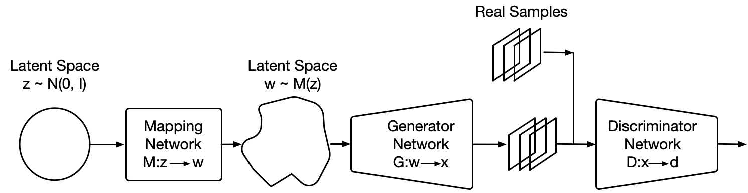
From generative models, Generative Adversarial Networks (GANs) have become increasingly popular, applied to different domains from imaging to signal processing. GANs (Goodfellow et al., 2014) are able to learn high fidelity and diverse data representations from a target distribution. This is done with a generator, $G(z)$ , that maps random noise, $\boldsymbol{z}\sim p_{\boldsymbol{z}}(z)$ , to samples that resemble the target data, $\boldsymbol{x}\sim p_{\text{ data }}(\boldsymbol{x})$ , and a discriminator, $D(x)$ , whose goal is to distinguish between real and generated samples. The goal of a GAN is find the equilibrium in the min-max problem:

\min_{G}\max_{D}V(D,G)=\mathbb{E}_{\boldsymbol{x}\sim p_{\text{ data }}(\boldsymbol{x})}[\log D(\boldsymbol{x})]+\mathbb{E}_{\boldsymbol{z}\sim p_{\boldsymbol{z}}(\boldsymbol{z})}[\log(1-D(G(\boldsymbol{z})))].

(1)

Since its introduction, modeling distributions of images has become the mainstream application for GANs, firstly introduced by Radford et al. (2015). State-of-the-art GANs such as BigGAN (Brock et al., 2019) and StyleGAN (Karras et al., 2019) have recently been use to generate impressive high-resolution images. Additionally, solutions like Spectral Normalization GANs (Miyato et al., 2018), Self-Attention GANs (Zhang et al., 2019a), and also BigGAN have achieved high diversity images in data sets like ImageNet (Deng et al., 2009), with 14 million images and 20 thousand different classes. At the same time, evaluating these models has been a challenging task. Many different metrics such as Inception Score (IS) (Salimans et al., 2016), Fréchet Inception Distance (FID) (Heusel et al., 2017), Maximum Mean Discrepancy (MMD) (Gretton et al., 2012), Kernel Inception Distance (KID) (Bińkowski et al., 2018), and 1-Nearest Neighbor classifier (1-NN) (Lopez-Paz and Oquab, 2016) have been proposed to do so, and thorough empirical studies (Huang et al., 2018; Barratt and Sharma, 2018) have shed some light on the advantages and disadvantages of each them. However, the selection of a feature space is crucial for using these metrics.

In our work we take a step towards developing a generative model that learns phenotypes through tissue architectures and cellular characteristics, introducing a GAN with representation learning properties and an interpretable latent space. We advocate that in the future these phenotype representations could give us insight about the diversity within/across cancer types and their relation to genomic, transcriptomic, and survival information; finally leading to better treatment and prognosis of the disease.

3 Methods

3.1 PathologyGAN

We used BigGAN (Brock et al., 2019) as a baseline architecture and introduced changes which empirically improved the Fréchet Inception Distance (FID) and the structure of the latent space.

BigGAN has been shown to be a successful GAN in replicating datasets with a diverse number of classes and large amounts of samples, such as ImageNet with approximately $1M$ samples and $20K$ classes. For this reason, we theorize that such model will be able to learn and replicate the diverse tissue phenotypes contained in whole slide images (WSI), being able to handle the large amount of tiles/patches resulting from diving the WSIs.

We followed the same architecture as BigGAN, employed Spectral Normalization in both generator and discriminator, self attention layers, and we also use orthogonal initialization and regularization as mentioned in the original paper.

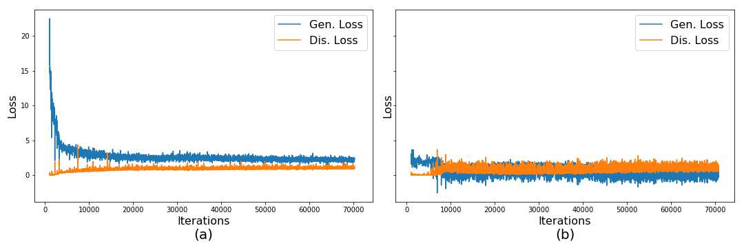
We make use of the Relativistic Average Discriminator (Jolicoeur-Martineau, 2019), where the discriminator’s goal is to estimate the probability of the real data being more realistic than the fake. We take this approach instead of following the Hinge loss (Lim and Ye, 2017) as the GAN objective. We find that this change makes the model convergence faster and produce higher quality images. Images using the Hinge loss did not capture the morphological structure of the tissue (we provide examples of these results in the Appendix C). The discriminator, and generator loss function are formulated as in Equations 2 and 3, where $\mathbb{P}$ is the distribution of real data, $\mathbb{Q}$ is the distribution for the fake data, and $C(x)$ is the non-transformed discriminator output or critic:

$\displaystyle L_{Dis}=-\mathbb{E}_{x_{r}\sim\mathbb{P}}$	$\displaystyle\left[\log\left(\tilde{D}\left(x_{r}\right)\right)\right]-\mathbb{E}_{x_{f}\sim\mathbb{Q}}\left[\log\left(1-\tilde{D}\left(x_{f}\right)\right)\right],$	(2)
$\displaystyle L_{Gen}=-\mathbb{E}_{x_{f}\sim\mathbb{Q}}$	$\displaystyle\left[\log\left(\tilde{D}\left(x_{f}\right)\right)\right]-\mathbb{E}_{x_{r}\sim\mathbb{P}}\left[\log\left(1-\tilde{D}\left(x_{r}\right)\right)\right],$	(3)
$\displaystyle\quad\quad\tilde{D}\left(x_{r}\right)$	$\displaystyle=\text{sigmoid}\left(C\left(x_{r}\right)-\mathbb{E}_{x_{f}\sim\mathbb{Q}}C\left(x_{f}\right)\right)),$	(4)
$\displaystyle\quad\quad\tilde{D}\left(x_{f}\right)$	$\displaystyle=\text{sigmoid}\left(C\left(x_{f}\right)-\mathbb{E}_{x_{r}\sim\mathbb{P}}C\left(x_{r}\right)\right).$	(5)

Additionally, we introduce two elements from StyleGAN (Karras et al., 2019) with the purpose of allowing the generator to freely optimize the latent space and find high-level features of the cancer tissue. First, a mapping network $M$ composed by four dense ResNet layers (He et al., 2016), placed after the latent vector $z\sim\mathcal{N}(0,I)$ , with the purpose of allowing the generator to find the latent space $w\sim M(z)$ that better disentangles the latent factors of variation. Secondly, style mixing regularization, where two different latent vectors $z1$ and $z2$ are run into the mapping network and fed at the same time to the generator, randomly choosing a layer in the generator and providing $w1$ and $w2$ to the different halves of the generator (e.g. on a generator of ten layers and being six the randomly selected layer, $w1$ would feed layers one to six and $w2$ seven to ten). Style mixing regularization encourages the generator to localize the high level features of the images in the latent space. We also use adaptive instance normalization (AdaIN) on our models, providing the entire latent vectors.

We use the Adam optimizer (Kingma and Ba, 2014) with $\beta_{1}=0.5$ and same learning rates of $0.0001$ for both generator and discriminator, the discriminator takes 5 steps for each of the generator. Each model was trained on an NVIDIA Titan RTX 24 GB for approximately 72 hours.

3.2 Datasets

To train our model, we used two different datasets, an H&E colorectal cancer tissue from the National Center for Tumor diseases (NCT, Germany) (Kather et al., 2018) and an H&E breast cancer tissue from the Netherlands Cancer Institute (NKI, Netherlands) and Vancouver General Hospital (VGH, Canada) (Beck et al., 2011).

The H&E breast cancer dataset was built from the Netherlands Cancer Institute (NKI) cohort and the Vancouver General Hospital (VGH) cohort with 248 and 328 patients, respectively. Each of them include TMA images, along with clinical patient data such as survival time, and estrogen-receptor (ER) status. The original TMA images all have a resolution of $1128\times 720$ pixels, and we split each of the images into smaller patches of $224\times 224$ , and allowed them to overlap by 50%. We also performed data augmentation on these images, a rotation of $90^{\circ}$ , and $180^{\circ}$ , and vertical and horizontal inversion. We filtered out images in which the tissue covers less than 70% of the area. In total this yield to a training set of 249K images and a test set of 62K.

The H&E colorectal cancer dataset provides 100K tissue images of $224\times 224$ resolution, each image has an associated type of tissue label: adipose, background, debris, lymphocytes, mucus, smooth muscle, normal colon mucosa, cancer-associated stroma, and colorectal adenocarcinoma epithelium (tumor). This dataset is composed of 86 H&E stained human cancer tissue slides. In order to check the model’s flexibility and ability to work with different datasets, we decided not to apply any data augmentation and use the tiles as they are provided.

In both datasets, we perform the partition over the total tissue patches, not according to patients, since our goal is to verify the ability to learn tissue representations. We trained our model on the VGH/NKI and NCT datasets for $45$ and $130$ epochs, respectively.

In Appendix B we study the model’s capacity in capturing representations with small size datasets (5K, 10K, 20K) verifying its converge and ability to generalize.

3.3 Evaluation metric on PathologyGAN

The Fréchet Inception Distance (FID) (Heusel et al., 2017) is a common metric used to measure GANs performance, and it quantifies the GAN’s ability to learn and reproduce the original data distribution. The goal of the FID score is to measure the similarity in quality and diversity between real $p_{data}(x)$ and generated data $p_{g}(x)$ .

Instead to measuring the distance between the real and generated distributions in the pixel space, it uses a pretrained ImageNet Inception Network (Szegedy et al., 2016) to extract features of each image, reducing the dimensionality of the samples and obtaining vision-relevant features. Feature samples are fitted into a multivariate Gaussian distribution obtaining real $\mathcal{N}(\mu_{data},\Sigma_{data})$ and generated $\mathcal{N}(\mu_{g},\Sigma_{g})$ feature distributions. Finally, it uses the Fréchet distance (Fréchet, 1957) to measure the difference between the two distributions:

FID=d^{2}((\mu_{data},\Sigma_{data}),(\mu_{g},\Sigma_{g}))=||\mu_{data}-\mu_{g}||^{2}_{2}+Tr(\Sigma_{data}+\Sigma_{g}-2(\Sigma_{data}\Sigma_{g})^{1/2})

We evaluate our model by calculating the FID score from $10K$ generated images and randomly sampling $10K$ real images.

We focus on using FID as it is a common GAN evaluation method (Brock et al., 2019; Karras et al., 2019; Miyato et al., 2018; Zhang et al., 2019a) that reliably captures differences between the real and generated distributions. Additionally, we provide more details in Appendix I comparing FID to other metrics such as Kernel Inception Distance (KID) or 1-Nearest Neighbor (1-NN) in the context of digital pathology.

3.4 Quantification of cancer cells in generated images - Breast cancer tissue

In our results, we use the counts of cancer cells and other cellular information as a mean to measure the image quality and representation learning properties of our model. The motivation behind this approach is to ensure that our model capture meaningful and faithful representations of the tissue.

We use this information in two different ways, first as an alternative feature space for FID as each image is translated into a vector with cellular information in the tissue, and secondly to label each generated tissue image according to the cancer cell density, allowing us to visualize the representation learning properties of our model’s latent space.

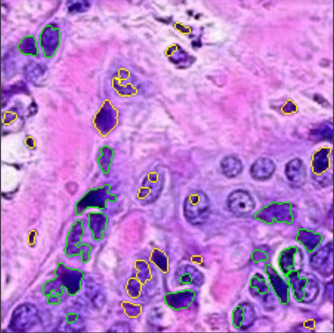
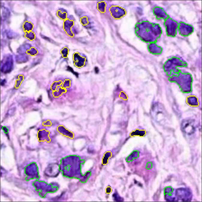
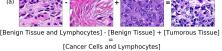
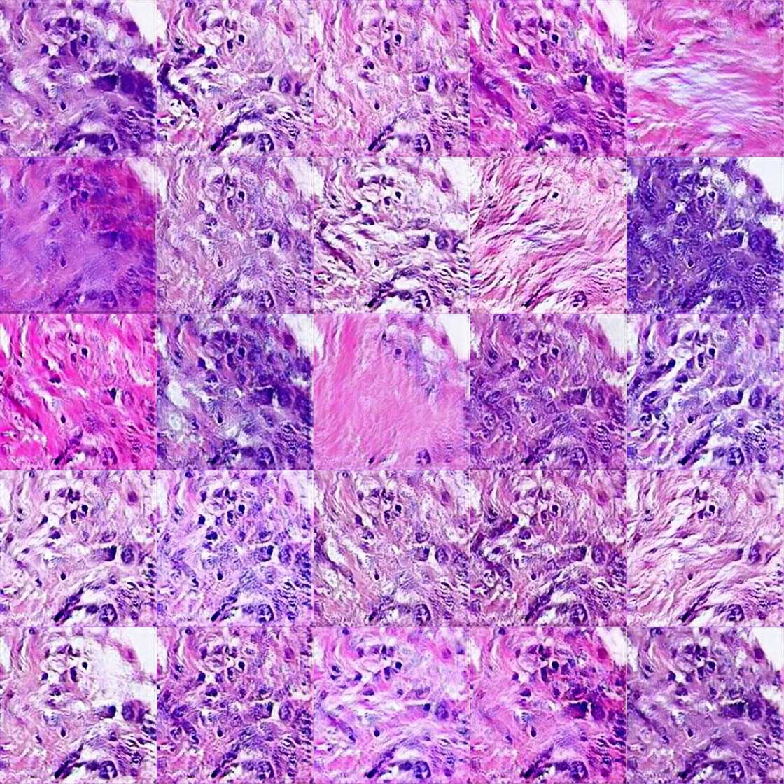
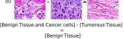
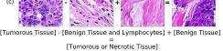
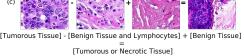
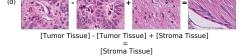
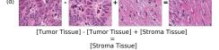
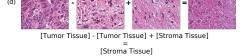
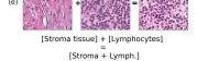
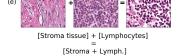
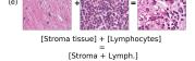
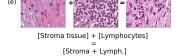
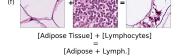
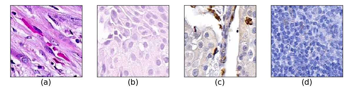
The CRImage tool (Yuan et al., 2012) uses an SVM classifier to provide quantitative information about tumor cellular characteristics in tissue. This approach allows us to gather pathological information in the images, namely the number of cancer cells, the number of other types of cells (such as stromal or lymphocytes), and the ratio of tumorous cells per area. We limit the use of this information to breast cancer tissue, since the tool was developed for this specific case. Figure 3 displays an example of how the CRImage captures the different cells in the generated images, such as cancer cells, stromal cells, and lymphocytes.

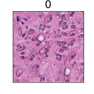
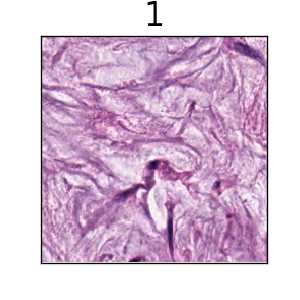
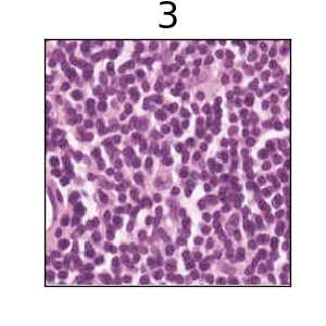
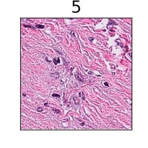
Finally, we created 8 different classes that account for counts of cancer cells in the tissue image, and consecutively we label each generated image with the corresponding class, allowing us to more clearly visualize the relation between cancer cell density in generated images and the model’s latent space.

Figure 3: CRImage identifies different cell types in our generated images. Cancer cells are highlighted with a green color, while lymphocytes and stromal cells are highlighted in yellow.

3.5 Tissue type assignation on generated images - Colorectal cancer tissue

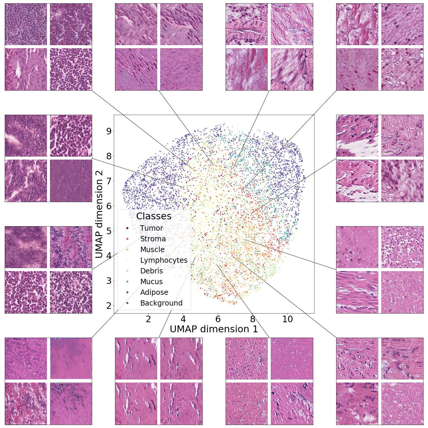
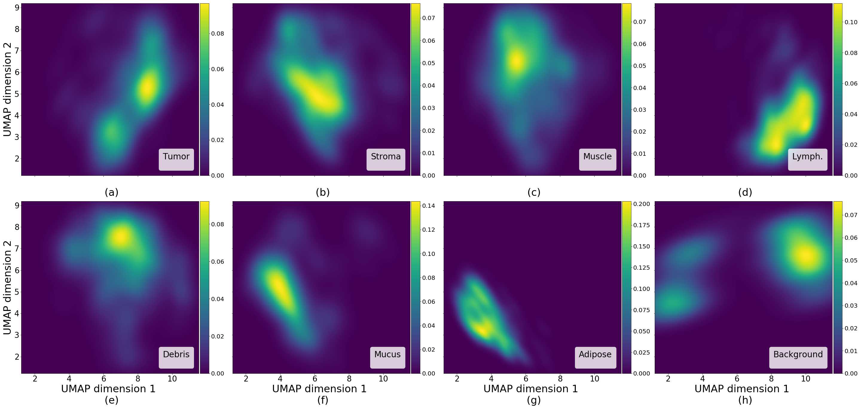
The NCT colorectal cancer dataset provides a label along each $224\times 224$ tissue sample and we make use of this information to label each generated image with a type of tissue, assigning a label to each generated image according to the 10-nearest neighbors of real images in the Inception-V1 feature space.

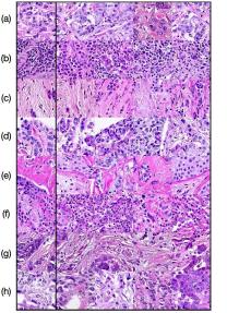
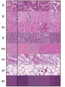
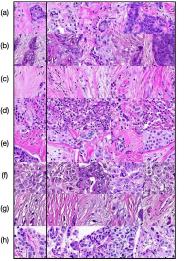
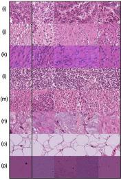
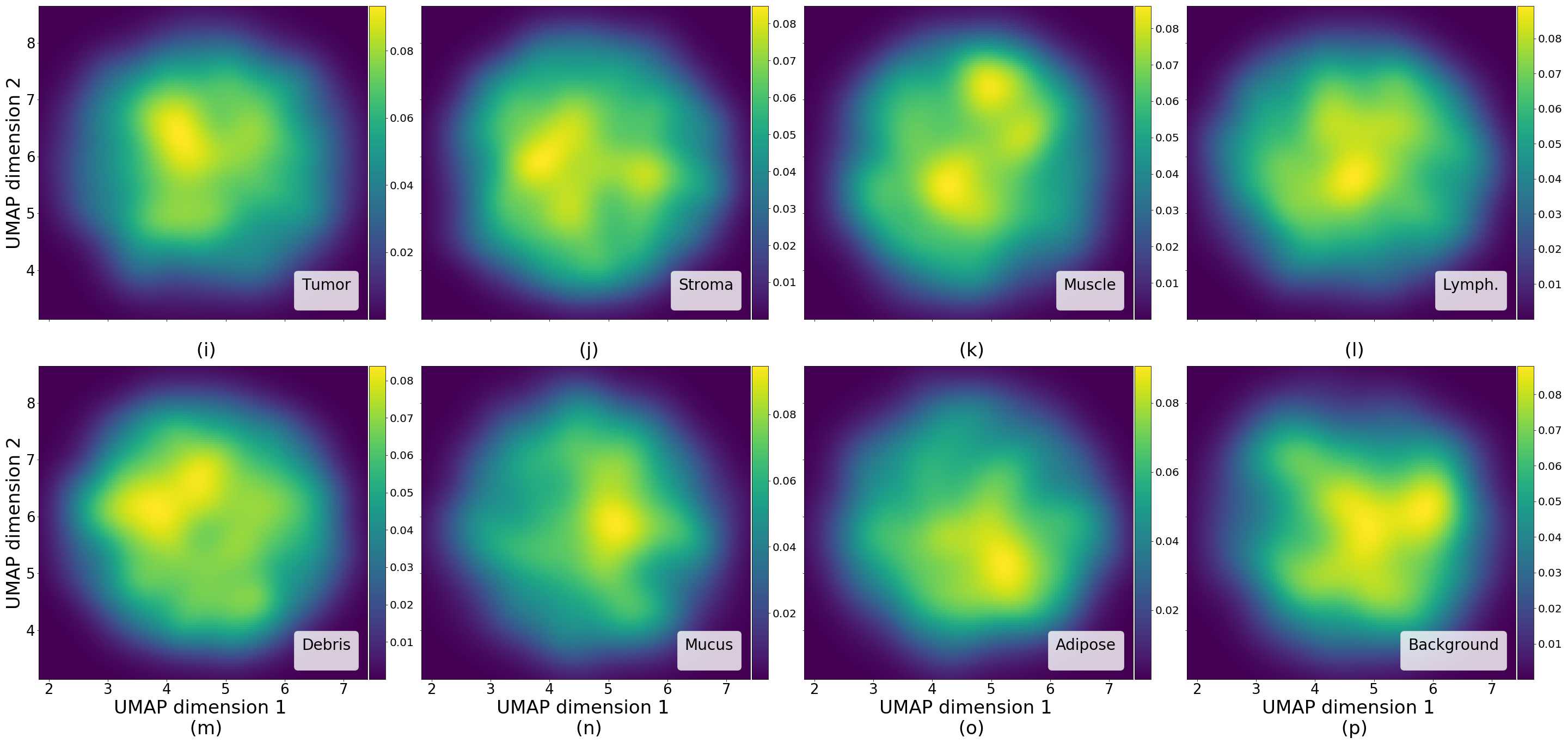
In Figure 4 we show generated images on the left column and the nearest real neighbors on the remaining columns. We present the different tissue types: tumor (i), stroma (j), muscle (k), lymphocytes (l), debris (m), mucus (n), adipose (o), and background (p). From this example, we can conclude that distance in feature space gives a good reference to find the tissue type of generated images.

4 Results

4.1 Image quality analysis

We study the fidelity of the generated images and their distribution in relation to the original data in two different ways, through measures of FID metrics and by visualizing the closest neighbors between generated and real images.

We calculate Fréchet Inception Distance (FID) with two different approaches, with the usual convolutional features of a Inception-V1 network and with cellular information extracted from the CRImage cell classifier, as explained in Section 3.4. We restrict using CRImage to breast cancer tissue only since it was developed for that particular purpose.

Table 1 shows that our model is able to achieve an accurate characterization of the cancer tissue. Using the Inception feature space, FID shows a stable representation for all models with values similar to ImageNet models of BigGAN (Brock et al., 2019) and SAGAN (Zhang et al., 2019a), with FIDs of 7.4 and 18.65, respectively or StyleGAN (Karras et al., 2019) trained on FFHQ with FID of 4.40. Using the CRImage cellular information as feature space, FID shows again close representations to real tissue.

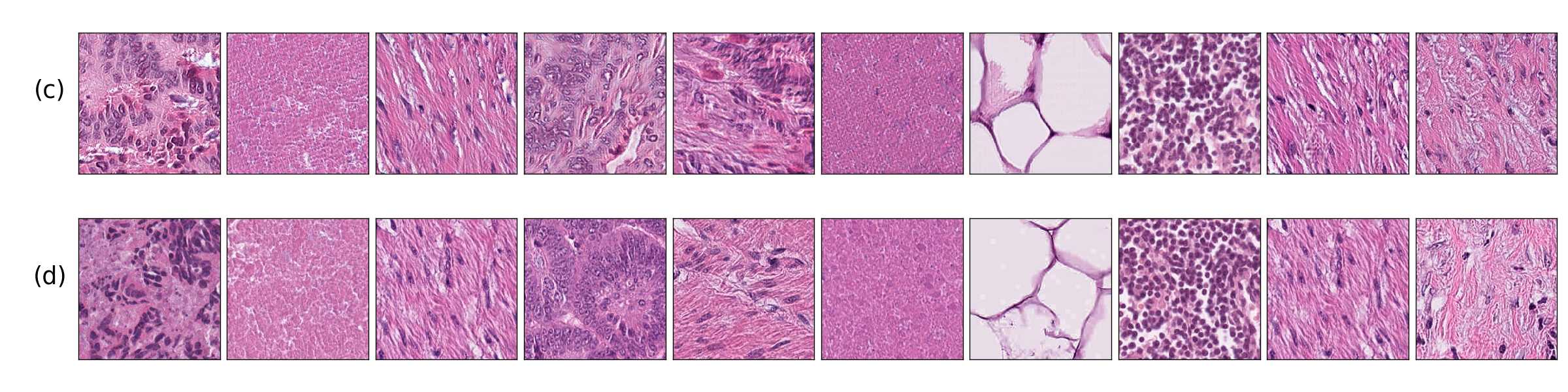
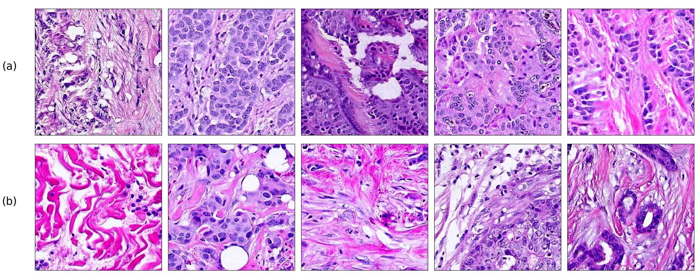
Additionally, in Figure 4 we present samples of generated images (first column) and its closest real neighbors in Inception-V1 feature space, the images are paired by rows. (a-h) correspond to different random samples of breast cancer tissue. In the case of colorectal cancer, we provide examples of different types of tissue: tumor (i), stroma (j), muscle (k), lymphocytes (l), debris (m), mucus (n), adipose (o), and background (p). We can see that generated and real images hold the same morphological characteristics.

Model	Inception FID	Inception FID	CRImage FID
	Colorectal	Breast	Breast
PathologyGAN	32.05 $\pm$ 3	16.65 $\pm$ 2.5	9.86 $\pm$ 0.4

Table 1: Evaluation of PathologyGANs. Mean and standard deviations are computed over three different random initializations. The low FID scores in both feature space suggest consistent and accurate representations.

4.2 Analysis of latent representations

In this section we focus on the PathologyGAN’s latent space, exploring the impact of introducing a mapping network in the generator and using style mixing regularization. Here we will provide examples of its impact on linear interpolations and vector operations on the latent space $w$ , as well as visualizations on the latent space $w$ . We conclude that PathologyGAN holds representation learning properties over cancer tissue morphologies.

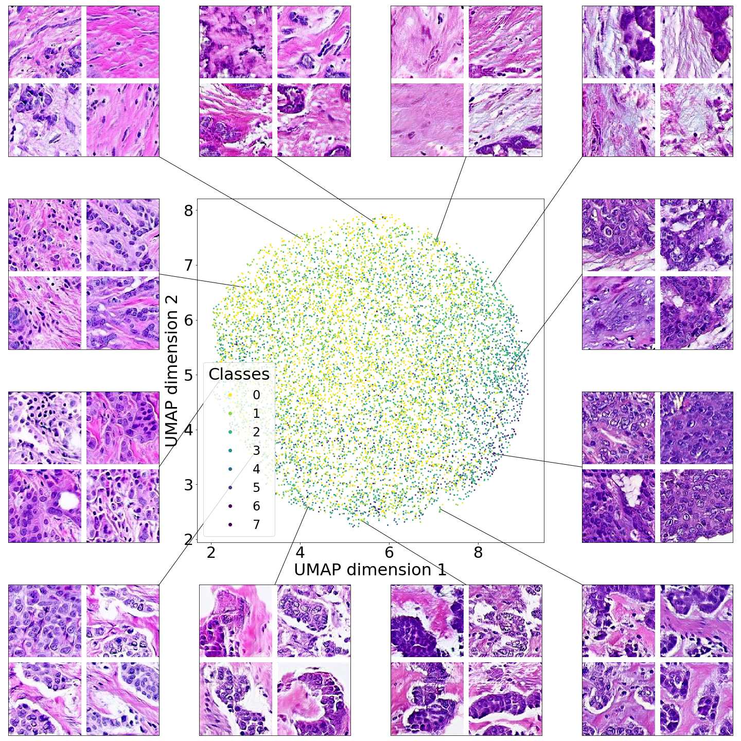
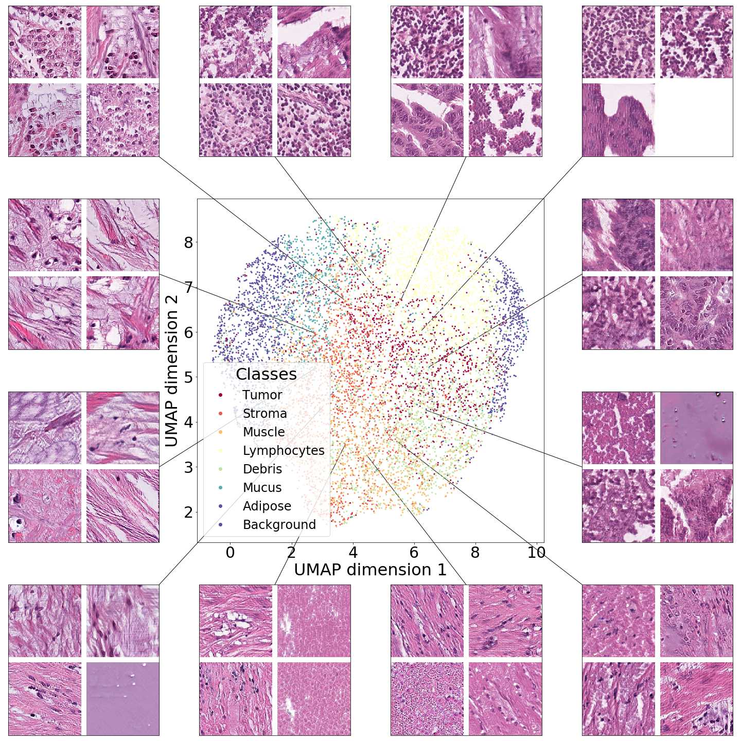
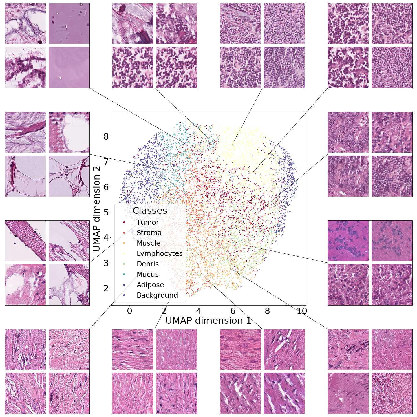
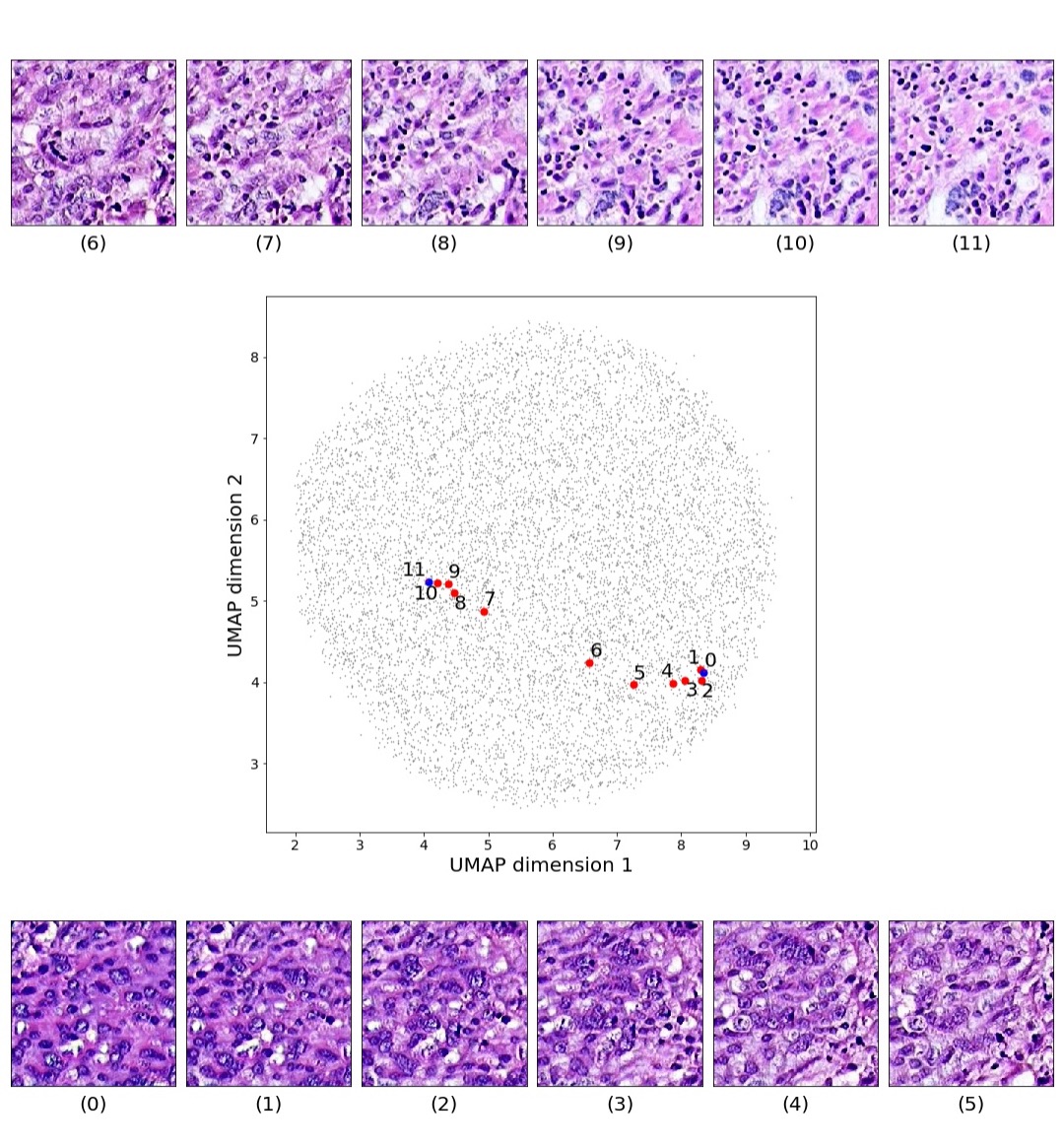
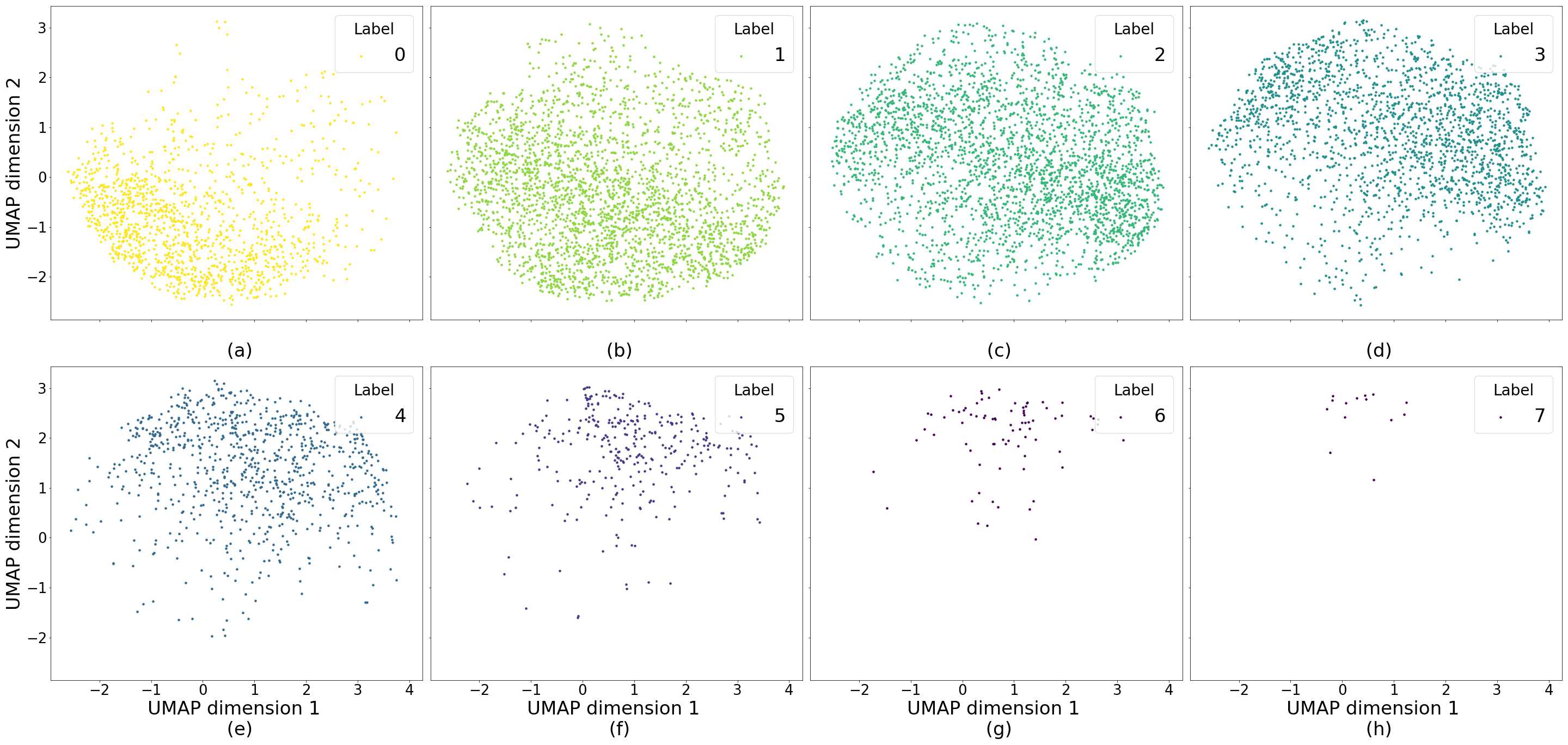
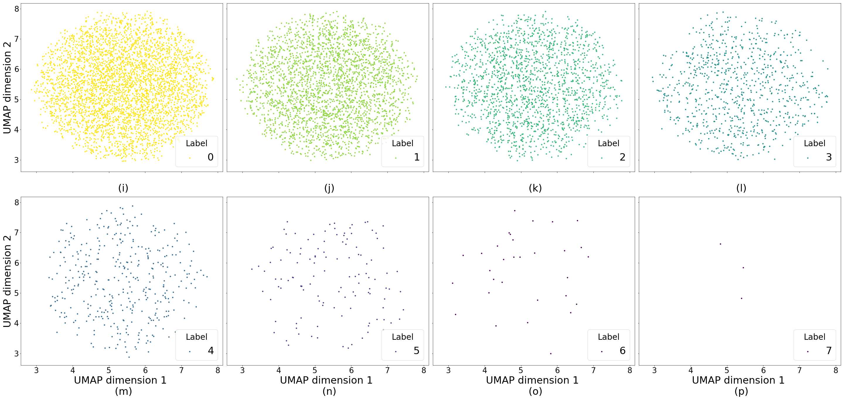
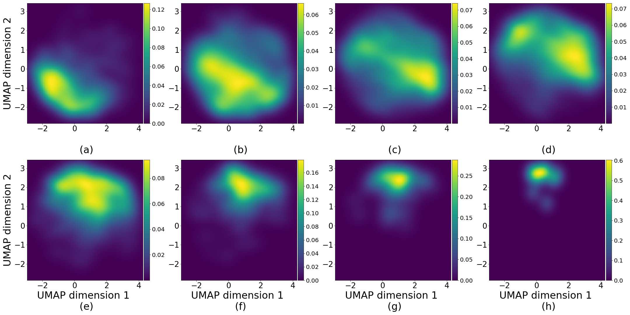
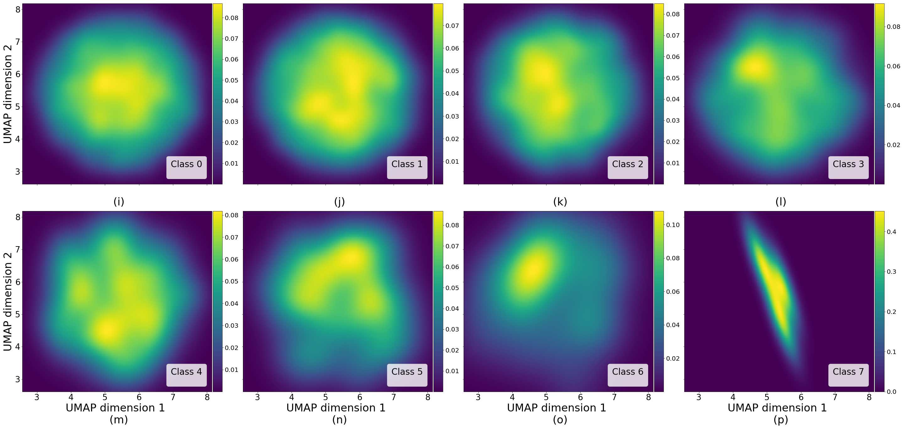
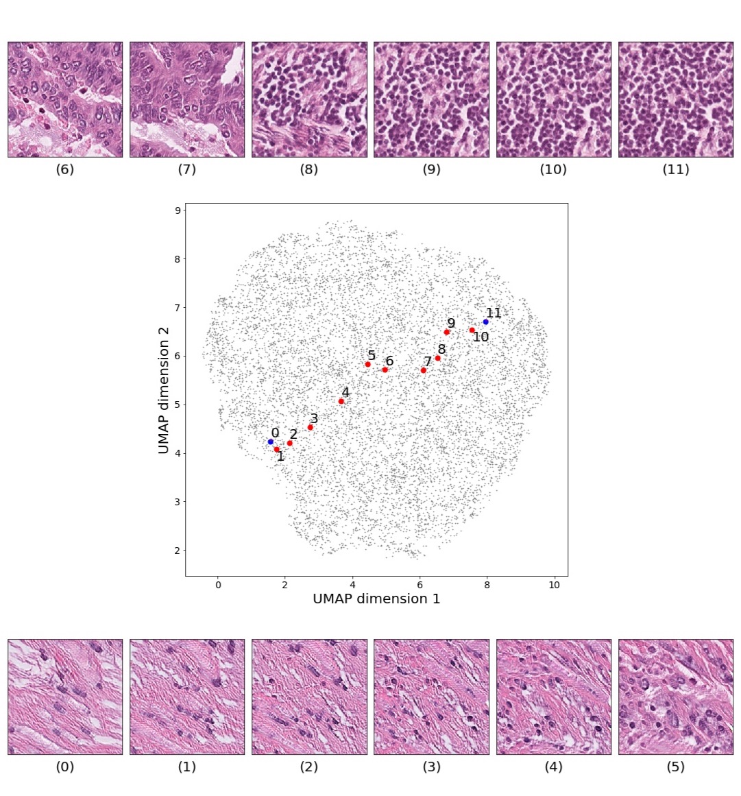
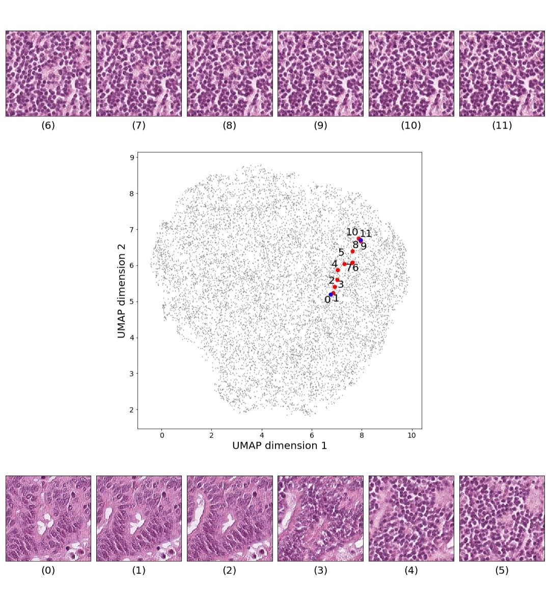
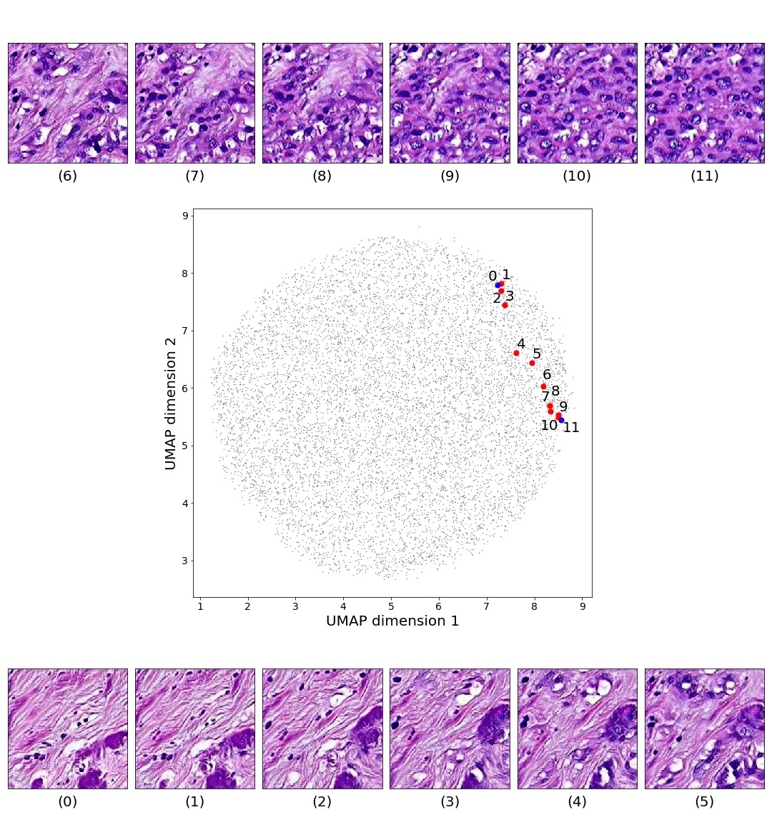
Figures 5 and 6 capture how the latent space $w$ has a structure that shows direct relationship with tissue properties. To create this figures, we generated $10K$ images and labeled them accordingly to Sections 3.4 and 3.5, along with each tissue image we also have the corresponding latent vector $w$ and we used UMAP (McInnes et al., 2018) to project them to a two dimensional space.

Figure 5 reveals the relationship between number of cancer cells in the breast cancer tissue and regions of the latent space, low counts of cancer cells (class 0) are concentrated at quadrant $II$ while they increase as we move to quadrant $IV$ (class 7). Figure 6 displays how the distinct regions of the latent space generate different kinds of tissue. These examples provide evidence of a structured latent space according to tissue cellular characteristics and tissue type. We include a further detailed exploration with density and scatter plots in the Appendix E.

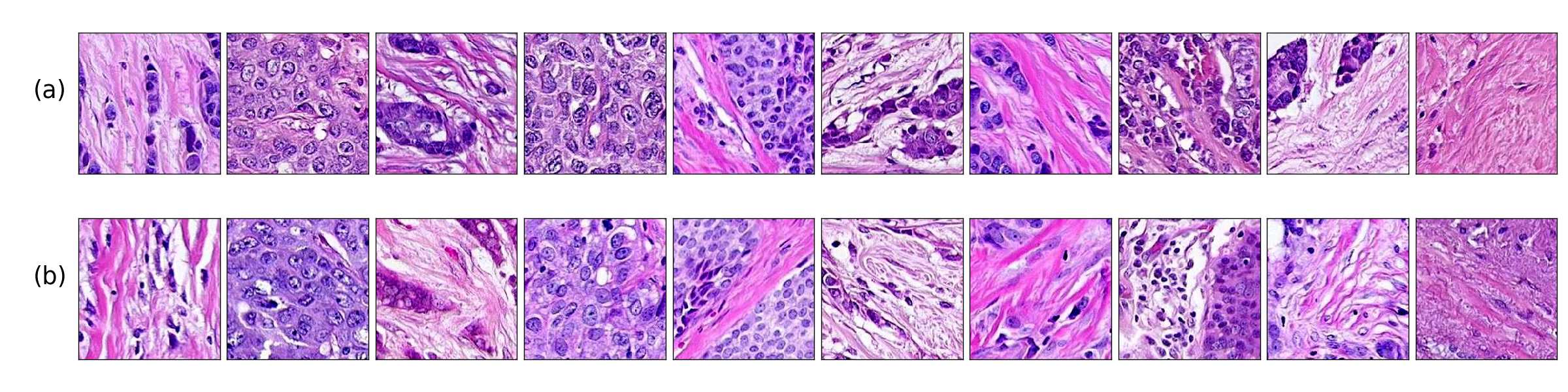
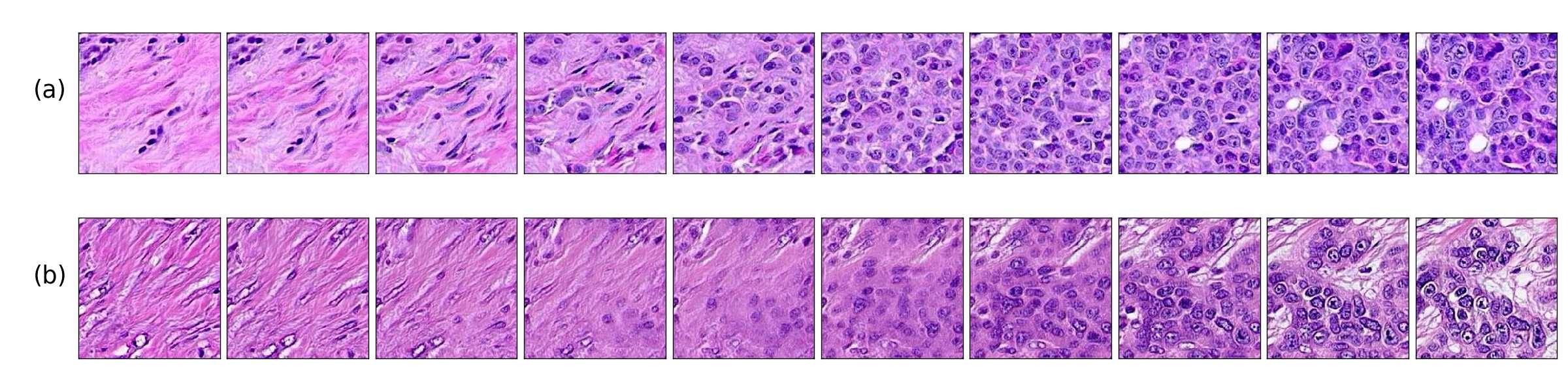
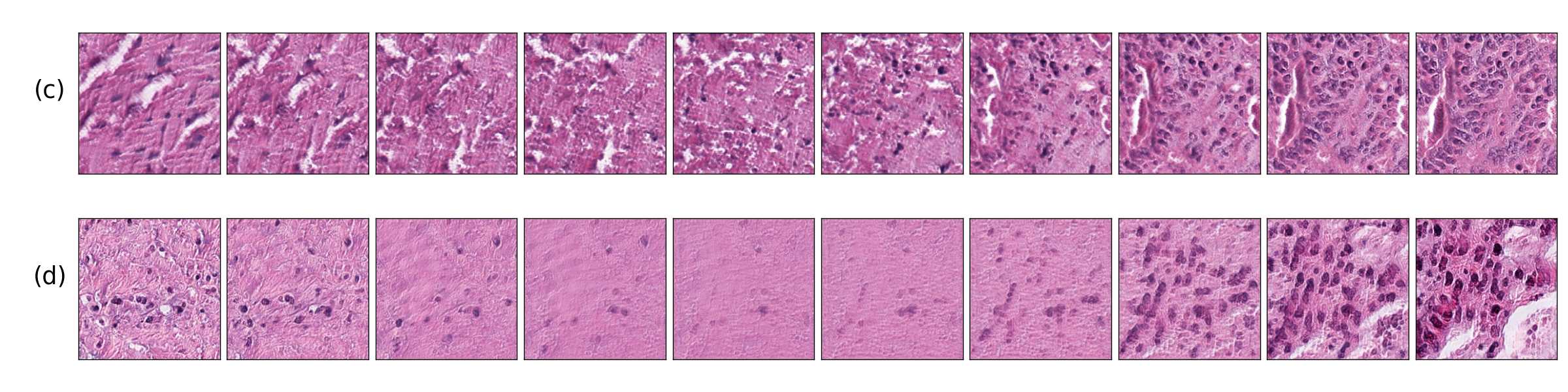
We also found that linear interpolations between two latent vectors $w$ have better feature transformations when the mapping network and style mixing regularization are introduced. Figure 7 shows linear interpolations in latent space $w$ between images with malignant tissue and benign tissue. (a, c) correspond to a model with a mapping network and style mixing regularization and (b, d) to a model without those features, we can see that transitions on (a, c) include an increasing population of cancer cells rather than the fading effect observed in images of (b, d). This result indicates that (a, c) better translates interpolations in the latent space, as real cells do not fade away.

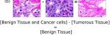
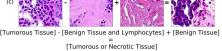
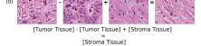
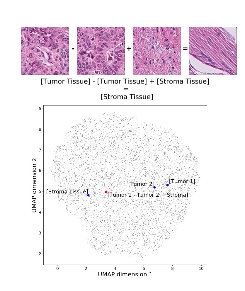
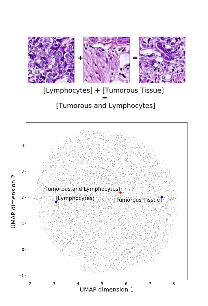
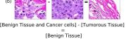
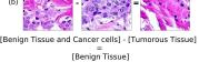
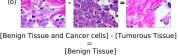
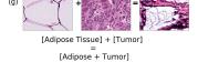
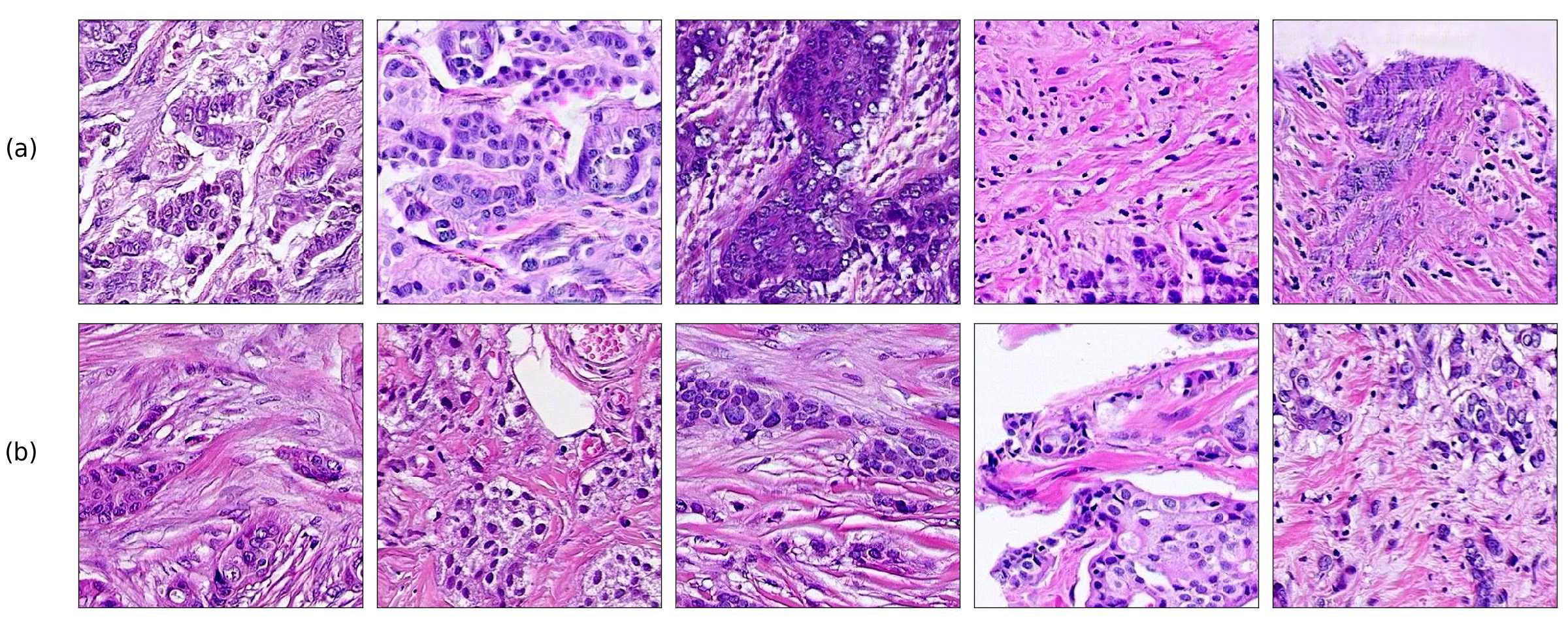
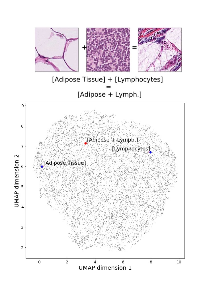
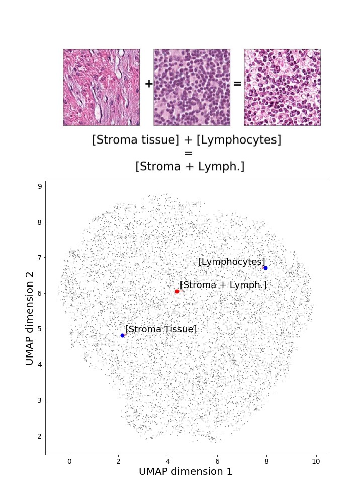
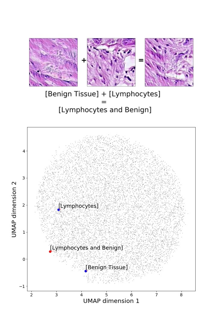
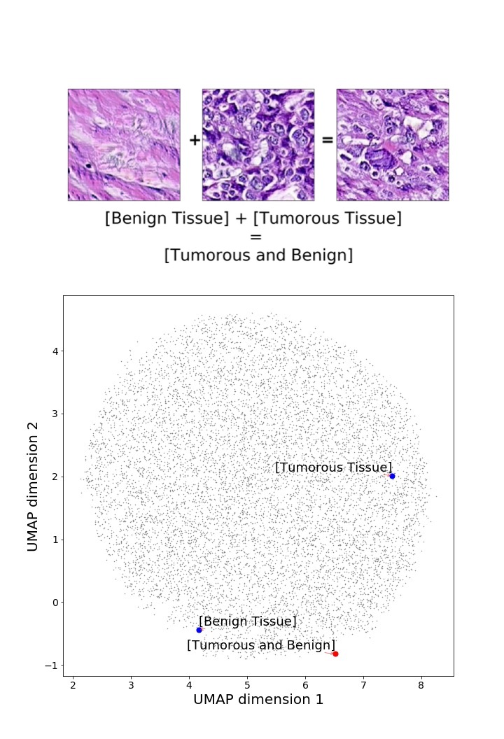
In addition, we performed linear vector operations in $w$ , that translated into semantic image features transformations. In Figure 8 we provide examples of three vector operations that result into feature alterations in the images. This evidence shows further support on the relation between a structured latent space and tissue characteristics.

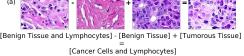
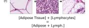
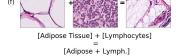
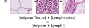
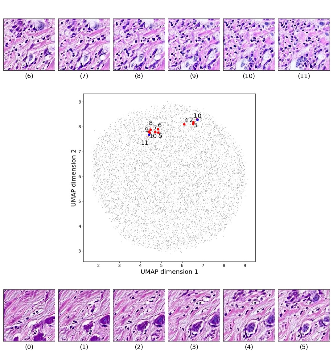
Finally, we explored how linear interpolation and vector operations translate into the individual points in the latent space. In Figure 9 we provide examples of interpolations from stroma to tumor in colorectal cancer, and tumor to lymphocytes in breast cancer. Through the intermediate vectors we show that gradual transitions in the latent space translate into smooth feature transformations, in these cases increase/decrease of tumorous cells or increase of lymphocyte counts. Alternatively, Figure 10 shows how results from vector operations fall into regions of the latent space that correspond to the expected tissue type or a combination of features such as tumor and lymphocytes. With these figures we visualize the meaningful representations of cells and tissue types, and also the interpretability of the latent space. Appendix H contains additional examples of these visualizations.

4.3 Pathologists’ results

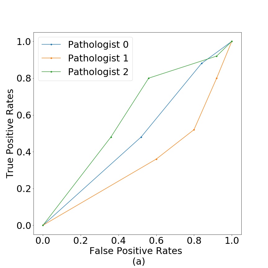
To demonstrate that the generated images can sustain the scrutiny of clinical examination, we asked expert pathologists to take a test, setup as follows:

•
50 Individual images - Pathologists were asked to rate all individual images from 1 to 5, where 5 meant the image appeared the most real.

We chose fake images in two ways, with half of them hand-selected and the other half with fake images that had the smallest Euclidean distance to real images in the convolutional feature space (Inception-V1). All the real images are randomly selected between the three closest neighbors of the fake images.

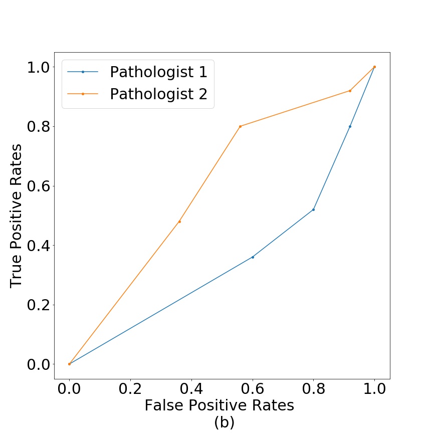
Figure 11 shows the test results in terms of false positive vs true positive for breast (a) and colorectal cancer tissue (b). We can see that pathologist classification is close to random. The pathologists mentioned that the usual procedure is to work with larger images with bigger resolution, but that the generated fake images were of a quality, that at the $224\times 224$ size used in this work, they were not able to differentiate between real and fake tissue.

5 Discussion

Our goal is to develop a generative model that is able to capture and create representations based tissue architectures and cellular characteristics that define phenotype, for this reason our results are focused on testing two features of our model: Image quality of generated tissue and interpretability of representations/structure of the latent space.

Through image quality we tested the model’s ability to learn and reproduce the distribution of tissue and cellular information, we argue that by doing so it would have capture phenotypes. The FID results on Table 1 show that PathologyGAN does reproduce these distributions not only when it is judged by convolutional features ( $32.05/16.65$ ) but also when we use an external tool to directly quantify cellular information in the tissue ( $9.86$ ). We would like to highlight that the FID score measures the distribution difference between real and generated samples, and given the low values we argue that the model is also capturing the abundance or scarcity of different tissue patterns.

Figure 4 shows generated tissue samples and their closest real neighbors in the Inception-V1 convolutional space, allowing us to visually inspect the similarity between them. In the colorectal cancer samples we can see that the different types of tissue (from tumor (i) to background (p)) clearly resemble the real tissue. Breast cancer tissue samples (a-h) also show the same result where the real and generated tissue present the same patterns and shapes.

As an additional image quality verification, we tested the generated images of our model against pathologists’ interpretation. We aimed to test that the generated tissues do not contain any artifacts that give them away as fake through the eyes of professionals. Given the near random classification between real/fake in Figure 11, we conclude that generated samples are realistic enough to pass as real through the examination of pathologists. We argue this is relevant because the model is able to reproduce tissue patterns to which pathologists are accustom to.

With the previous results we conclude that the model is able to reproduce the detail and distribution of tissue, not only from the convolutional features or cellular characteristics perspective, but also by the interpretation of pathologists.

In relation to PathologyGAN’s latent space structure and interpretability of its representations, Figures 5 and 6 show how distinct regions of the latent space hold tissue and cellular information about the generated images. Figure 5 shows a clear relationship between regions of the latent space and the cancer cell density in the tissue, while Figure 6 directly links the region of the space with the different tissue types (e.g. tumor, stroma, muscle, lymphocytes, debris, mucus, adipose, and background). In Figures 7 and 9 we relate linear interpolations between latent vectors and generated tissue attributes, showing that gradual transitions in the latent space transfer into smooth feature transformations, in these cases increase/decrease of tumorous cells or increase of lymphocyte counts. Finally, Figures 8 and 10 provide examples of linear vector operations and their translation into tissue characteristic changes, with different tissue changes. These results provide support on the representation learning properties of the model, not only holding meaningful information of cell and tissue types but also an interpretable insight to the representations themselves.

As future research, we consider that our model could be used in different settings. PathologyGAN could be extended to achieve higher resolutions such as $1024\times 1024$ , a level of resolution which could include complete TMAs which hold value for diagnosis and prognosis. In these cases, pathologists’ insight will hold a higher value, since they are used to working at WSI or TMA level. In addition, the study with pathologists could be extended to include a larger number of experts and to use a random sample of generated images which would give a less biased result.

The representation learning properties of the model can also contribute as a educational tool, providing tissue samples with certain cellular characteristics that are rare, elucidating possible transitions of tissue (e.g. from tumor to high lymphocyte infiltration), or enabling the study of borderline cases (e.g. atypia) between generated images and pathologists interpretations.

Furthermore, the model could be used to generate synthetic samples to improve classifiers performance, helping to avoid overfitting and providing samples with rare tissue pathologies.

Finally, we consider the model can contribute to characterizing phenotype patterns, creating representations by cellular and tissue morphologies, this is where we think the tissue representation learning properties are key. Linking these phenotypes to patient related information such as genomic, transcriptomic information, or survival expectancy. Ultimately this could give insight to the tumor microenvironment recorded in the WSIs and a better understanding of the disease. In order to achieve this goal, it will require exploring the addition of an encoder to map real images into the GAN’s latent space (Quiros et al., 2020) and verify its converge when large amounts of samples are used, since WSIs in datasets like TCGA could amount to millions of tissue samples.

6 Conclusion

We presented a new approach to the use of machine learning in digital pathology, using GANs to learn cancer tissue representations. We assessed the quality of the generated images through the FID metric, using the convolutional features of a Inception-V1 network and quantitative cellular information of the tissue, both showed consistent state-of-the-art values for different kinds of tissue, breast and colorectal cancer. We showed that our model allows high level interpretation of its latent space, even performing linear operations that translate into feature tissue transformations. Finally, we demonstrate that the quality of the generated images do not allow pathologists to reliably find differences between real and generated images.

With PathologyGAN we proposed a generative model that captures representations of entire tissue architectures and defines an interpretable latent space (e.g. colour, texture, spatial features of cancer and normal cells, and their interaction), contributing to generative models ability to capture phenotype representations.

Acknowledgments

We would like to thank Joanne Edwards, Christopher Bigley, and Elizabeth Mallon for helpful insights and discussions on this work.

We will also like to acknowledge funding support from University of Glasgow on A.C.Q scholarship, K.Y from EPSRC grant EP/R018634/1., and R.M-S. from EPSRC grants EP/T00097X/1 and EP/R018634/1.

Ethical Standards

The work follows appropriate ethical standards in conducting research and writing the manuscript. Our models were trained with publicly available data, for which no ethical approval was required.

Conflicts of Interest

We declare we don’t have conflicts of interest.

References

Barratt and Sharma (2018) Shane Barratt and Rishi Sharma. A note on the Inception score. CoRR, abs/1801.01973, 2018. URL http://arxiv.org/abs/1801.01973.
Beck et al. (2011) Andrew H Beck, Ankur R Sangoi, Samuel Leung, Robert J Marinelli, Torsten O Nielsen, Marc J van de Vijver, Robert B West, Matt van de Rijn, and Daphne Koller. Systematic analysis of breast cancer morphology uncovers stromal features associated with survival. Sci Transl Med, 3(108):108ra113, Nov 2011. ISSN 1946-6242 (Electronic); 1946-6234 (Linking). doi: 10.1126/scitranslmed.3002564.
Bergenstråhle et al. (2020a) Joseph Bergenstråhle, Ludvig Larsson, and Joakim Lundeberg. Seamless integration of image and molecular analysis for spatial transcriptomics workflows. BMC Genomics, 21(1):482, 2020a. doi: 10.1186/s12864-020-06832-3. URL https://doi.org/10.1186/s12864-020-06832-3.
Bergenstråhle et al. (2020b) Ludvig Bergenstråhle, Bryan He, Joseph Bergenstråhle, Alma Andersson, Joakim Lundeberg, James Zou, and Jonas Maaskola. Super-resolved spatial transcriptomics by deep data fusion. bioRxiv, page 2020.02.28.963413, 01 2020b.
Bińkowski et al. (2018) Mikołaj Bińkowski, Dougal J. Sutherland, Michael Arbel, and Arthur Gretton. Demystifying MMD GANs. In International Conference on Learning Representations, 2018. URL https://openreview.net/forum?id=r1lUOzWCW.
Brock et al. (2019) Andrew Brock, Jeff Donahue, and Karen Simonyan. Large scale GAN training for high fidelity natural image synthesis. In International Conference on Learning Representations, 2019. URL https://openreview.net/forum?id=B1xsqj09Fm.
Campbell et al. (2020) Peter J. Campbell, Gad Getz, Jan O. Korbel, and et al. Pan-cancer analysis of whole genomes. Nature, 578(7793):82–93, 2020.
Coudray and Tsirigos (2020) Nicolas Coudray and Aristotelis Tsirigos. Deep learning links histology, molecular signatures and prognosis in cancer. Nature Cancer, 1(8):755–757, 2020. doi: 10.1038/s43018-020-0099-2. URL https://doi.org/10.1038/s43018-020-0099-2.
Coudray et al. (2018) Nicolas Coudray, Paolo Santiago Ocampo, Theodore Sakellaropoulos, Navneet Narula, Matija Snuderl, David Fenyö, Andre L. Moreira, Narges Razavian, and Aristotelis Tsirigos. Classification and mutation prediction from non–small cell lung cancer histopathology images using deep learning. Nature Medicine, 24(10):1559–1567, 2018. doi: 10.1038/s41591-018-0177-5. URL https://doi.org/10.1038/s41591-018-0177-5.
de Bel et al. (2018) Thomas de Bel, Meyke Hermsen, Bart Smeets, Luuk Hilbrands, Jeroen van der Laak, and Geert Litjens. Automatic segmentation of histopathological slides of renal tissue using deep learning. In Medical Imaging 2018: Digital Pathology, volume 10581, page 1058112. International Society for Optics and Photonics, 2018.
Deng et al. (2009) J. Deng, W. Dong, R. Socher, L.-J. Li, K. Li, and L. Fei-Fei. ImageNet: A Large-Scale Hierarchical Image Database. In CVPR09, 2009.
Dentro et al. (2020) Stefan C. Dentro, Ignaty Leshchiner, and et al. Characterizing genetic intra-tumor heterogeneity across 2,658 human cancer genomes. bioRxiv, 2020. doi: 10.1101/312041. URL https://www.biorxiv.org/content/early/2020/04/22/312041.
Fréchet (1957) Maurice Fréchet. Sur la distance de deux lois de probabilité. COMPTES RENDUS HEBDOMADAIRES DES SEANCES DE L ACADEMIE DES SCIENCES, 244(6):689–692, 1957.
Fu et al. (2020) Yu Fu, Alexander W. Jung, Ramon Viñas Torne, Santiago Gonzalez, Harald Vöhringer, Artem Shmatko, Lucy R. Yates, Mercedes Jimenez-Linan, Luiza Moore, and Moritz Gerstung. Pan-cancer computational histopathology reveals mutations, tumor composition and prognosis. Nature Cancer, 1(8):800–810, 2020. doi: 10.1038/s43018-020-0085-8. URL https://doi.org/10.1038/s43018-020-0085-8.
Gadermayr et al. (2018) Michael Gadermayr, Laxmi Gupta, Barbara M Klinkhammer, Peter Boor, and Dorit Merhof. Unsupervisedly training gans for segmenting digital pathology with automatically generated annotations. arXiv preprint arXiv:1805.10059, 2018.
Gadermayr et al. (2019) Michael Gadermayr, Laxmi Gupta, Vitus Appel, Peter Boor, Barbara M Klinkhammer, and Dorit Merhof. Generative adversarial networks for facilitating stain-independent supervised and unsupervised segmentation: a study on kidney histology. IEEE transactions on medical imaging, 38(10):2293–2302, 2019.
Gerstung et al. (2020) Moritz Gerstung, Clemency Jolly, and et al. The evolutionary history of 2,658 cancers. Nature, 578(7793):122–128, 2020.
Goodfellow et al. (2014) Ian Goodfellow, Jean Pouget-Abadie, Mehdi Mirza, Bing Xu, David Warde-Farley, Sherjil Ozair, Aaron Courville, and Yoshua Bengio. Generative adversarial nets. In Z. Ghahramani, M. Welling, C. Cortes, N. D. Lawrence, and K. Q. Weinberger, editors, Advances in Neural Information Processing Systems 27, pages 2672–2680. Curran Associates, Inc., 2014. URL http://papers.nips.cc/paper/5423-generative-adversarial-nets.pdf.
Gretton et al. (2012) Arthur Gretton, Karsten M. Borgwardt, Malte J. Rasch, Bernhard Schölkopf, and Alexander Smola. A kernel two-sample test. Journal of Machine Learning Research, 13(25):723–773, 2012. URL http://jmlr.org/papers/v13/gretton12a.html.
He et al. (2020) Bryan He, Ludvig Bergenstråhle, Linnea Stenbeck, Abubakar Abid, Alma Andersson, Åke Borg, Jonas Maaskola, Joakim Lundeberg, and James Zou. Integrating spatial gene expression and breast tumour morphology via deep learning. Nature Biomedical Engineering, 4(8):827–834, 2020. doi: 10.1038/s41551-020-0578-x. URL https://doi.org/10.1038/s41551-020-0578-x.
He et al. (2016) Kaiming He, Xiangyu Zhang, Shaoqing Ren, and Jian Sun. Deep residual learning for image recognition. 2016 IEEE Conference on Computer Vision and Pattern Recognition (CVPR), Jun 2016. doi: 10.1109/cvpr.2016.90. URL http://dx.doi.org/10.1109/cvpr.2016.90.
Heusel et al. (2017) Martin Heusel, Hubert Ramsauer, Thomas Unterthiner, Bernhard Nessler, and Sepp Hochreiter. Gans trained by a two time-scale update rule converge to a local nash equilibrium. In I. Guyon, U. V. Luxburg, S. Bengio, H. Wallach, R. Fergus, S. Vishwanathan, and R. Garnett, editors, Advances in Neural Information Processing Systems 30, pages 6626–6637. Curran Associates, Inc., 2017.
Hou et al. (2019) Le Hou, Vu Nguyen, Ariel B Kanevsky, Dimitris Samaras, Tahsin M Kurc, Tianhao Zhao, Rajarsi R Gupta, Yi Gao, Wenjin Chen, David Foran, and Joel H Saltz. Sparse autoencoder for unsupervised nucleus detection and representation in histopathology images. Pattern recognition, 86:188–200, 02 2019. doi: 10.1016/j.patcog.2018.09.007. URL https://pubmed.ncbi.nlm.nih.gov/30631215.
Hu et al. (2019) Bo Hu, Ye Tang, Eric I-Chao Chang, Yubo Fan, Maode Lai, and Yan Xu. Unsupervised learning for cell-level visual representation in histopathology images with generative adversarial networks. IEEE Journal of Biomedical and Health Informatics, 23(3):1316–1328, May 2019. ISSN 2168-2208. doi: 10.1109/jbhi.2018.2852639. URL http://dx.doi.org/10.1109/JBHI.2018.2852639.
Huang et al. (2018) Gao Huang, Yang Yuan, Qiantong Xu, Chuan Guo, Yu Sun, Felix Wu, and Kilian Weinberger. An empirical study on evaluation metrics of generative adversarial networks, 2018. URL https://openreview.net/forum?id=Sy1f0e-R-.
Jolicoeur-Martineau (2019) Alexia Jolicoeur-Martineau. The relativistic discriminator: a key element missing from standard GAN. In International Conference on Learning Representations, 2019. URL https://openreview.net/forum?id=S1erHoR5t7.
Karras et al. (2019) Tero Karras, Samuli Laine, and Timo Aila. A style-based generator architecture for generative adversarial networks. 2019 IEEE/CVF Conference on Computer Vision and Pattern Recognition (CVPR), Jun 2019. doi: 10.1109/cvpr.2019.00453. URL http://dx.doi.org/10.1109/CVPR.2019.00453.
Kather et al. (2018) Jakob Nikolas Kather, Niels Halama, and Alexander Marx. 100,000 histological images of human colorectal cancer and healthy tissue, April 2018. URL https://doi.org/10.5281/zenodo.1214456.
Kather et al. (2020) Jakob Nikolas Kather, Lara R. Heij, Heike I. Grabsch, and et al. Pan-cancer image-based detection of clinically actionable genetic alterations. Nature Cancer, 1(8):789–799, 2020. doi: 10.1038/s43018-020-0087-6. URL https://doi.org/10.1038/s43018-020-0087-6.
Katzman et al. (2018) Jared L. Katzman, Uri Shaham, Alexander Cloninger, Jonathan Bates, Tingting Jiang, and Yuval Kluger. Deepsurv: personalized treatment recommender system using a cox proportional hazards deep neural network. BMC Medical Research Methodology, 18(1), Feb 2018. ISSN 1471-2288. doi: 10.1186/s12874-018-0482-1. URL http://dx.doi.org/10.1186/s12874-018-0482-1.
Kingma and Ba (2014) Diederik P Kingma and Jimmy Ba. Adam: A method for stochastic optimization. arXiv preprint arXiv:1412.6980, 2014.
Lee et al. (2018) C. Lee, W. Zame, Jinsung Yoon, and M. V. D. Schaar. Deephit: A deep learning approach to survival analysis with competing risks. In AAAI, 2018.
Levine et al. (2020) Adrian B Levine, Jason Peng, David Farnell, Mitchell Nursey, and et al. Synthesis of diagnostic quality cancer pathology images by generative adversarial networks. The Journal of Pathology, 252(2):178–188, 2020. doi: https://doi.org/10.1002/path.5509. URL https://onlinelibrary.wiley.com/doi/abs/10.1002/path.5509.
Lim and Ye (2017) Jae Hyun Lim and Jong Chul Ye. Geometric GAN, 2017.
Lopez-Paz and Oquab (2016) David Lopez-Paz and Maxime Oquab. Revisiting classifier two-sample tests, 2016.
Mahmood et al. (2018) Faisal Mahmood, Daniel Borders, Richard Chen, Gregory McKay, Kevan J Salimian, Alexander Baras, and Nicholas Durr. Deep adversarial training for multi-organ nuclei segmentation in histopathology images, 09 2018.
Marinelli et al. (2008) Robert J. Marinelli, Kelli Montgomery, Chih Long Liu, Nigam Shah, Wijan Prapong, Michael Nitzberg, Zachariah K Zachariah, Gavin Sherlock, Yasodha Natkunam, Robert B West, Matt van de Rijn, Patrick O Brown, and Catherine A Ball. The stanford tissue microarray database. Nucleic acids research, 36:D871–7, 02 2008. doi: 10.1093/nar/gkm861.
McInnes et al. (2018) Leland McInnes, John Healy, Nathaniel Saul, and Lukas Großberger. UMAP: Uniform Manifold Approximation and Projection. Journal of Open Source Software, 3(29), 2018.
Miyato et al. (2018) Takeru Miyato, Toshiki Kataoka, Masanori Koyama, and Yuichi Yoshida. Spectral normalization for generative adversarial networks. In International Conference on Learning Representations, 2018. URL https://openreview.net/forum?id=B1QRgziT-.
Qaiser et al. (2019) Talha Qaiser, Yee-Wah Tsang, Daiki Taniyama, Naoya Sakamoto, Kazuaki Nakane, David Epstein, and Nasir Rajpoot. Fast and accurate tumor segmentation of histology images using persistent homology and deep convolutional features. Medical image analysis, 55:1–14, 2019.
Qu et al. (2019) Hui Qu, Gregory Riedlinger, Pengxiang Wu, Qiaoying Huang, Jingru Yi, Subhajyoti De, and Dimitris Metaxas. Joint segmentation and fine-grained classification of nuclei in histopathology images. In 2019 IEEE 16th International Symposium on Biomedical Imaging (ISBI 2019), pages 900–904. IEEE, 2019.
Quiros et al. (2020) Adalberto Claudio Quiros, Roderick Murray-Smith, and Ke YuCoudan. Learning a low dimensional manifold of real cancer tissue with pathologygan, 2020.
Radford et al. (2015) Alec Radford, Luke Metz, and Soumith Chintala. Unsupervised representation learning with deep convolutional generative adversarial networks, 2015.
Rana et al. (2018) Aman Rana, Gregory Yauney, Alarice Lowe, and Pratik Shah. Computational histological staining and destaining of prostate core biopsy RGB images with Generative Adversarial Neural Networks. 2018 17th IEEE International Conference on Machine Learning and Applications (ICMLA), Dec 2018. doi: 10.1109/icmla.2018.00133. URL http://dx.doi.org/10.1109/ICMLA.2018.00133.
Salimans et al. (2016) Tim Salimans, Ian Goodfellow, Wojciech Zaremba, Vicki Cheung, Alec Radford, Xi Chen, and Xi Chen. Improved techniques for training gans. In D. D. Lee, M. Sugiyama, U. V. Luxburg, I. Guyon, and R. Garnett, editors, Advances in Neural Information Processing Systems 29, pages 2234–2242. Curran Associates, Inc., 2016. URL http://papers.nips.cc/paper/6125-improved-techniques-for-training-gans.pdf.
Schmauch et al. (2020) Benoît Schmauch, Alberto Romagnoni, Elodie Pronier, Charlie Saillard, Pascale Maillé, Julien Calderaro, Aurélie Kamoun, Meriem Sefta, Sylvain Toldo, Mikhail Zaslavskiy, Thomas Clozel, Matahi Moarii, Pierre Courtiol, and Gilles Wainrib. A deep learning model to predict rna-seq expression of tumours from whole slide images. Nature Communications, 11(1):3877, 2020. doi: 10.1038/s41467-020-17678-4. URL https://doi.org/10.1038/s41467-020-17678-4.
Szegedy et al. (2016) C. Szegedy, V. Vanhoucke, S. Ioffe, J. Shlens, and Z. Wojna. Rethinking the inception architecture for computer vision. In 2016 IEEE Conference on Computer Vision and Pattern Recognition (CVPR), pages 2818–2826, 2016. doi: 10.1109/CVPR.2016.308.
Tellez et al. (2018) David Tellez, Maschenka Balkenhol, Irene Otte-Höller, Rob van de Loo, Rob Vogels, Peter Bult, Carla Wauters, Willem Vreuls, Suzanne Mol, Nico Karssemeijer, et al. Whole-slide mitosis detection in h&e breast histology using phh3 as a reference to train distilled stain-invariant convolutional networks. IEEE transactions on medical imaging, 37(9):2126–2136, 2018.
Vickovic et al. (2019) Sanja Vickovic, Gökcen Eraslan, Fredrik Salmén, and et al. High-definition spatial transcriptomics for in situ tissue profiling. Nature Methods, 16(10):987–990, 2019.
Wang et al. (2020) Yuliang Wang, Shuyi Ma, and Walter L. Ruzzo. Spatial modeling of prostate cancer metabolic gene expression reveals extensive heterogeneity and selective vulnerabilities. Scientific Reports, 10(1):3490, 2020. doi: 10.1038/s41598-020-60384-w. URL https://doi.org/10.1038/s41598-020-60384-w.
Wei et al. (2019) Jason W. Wei, Laura J. Tafe, Yevgeniy A. Linnik, Louis J. Vaickus, Naofumi Tomita, and Saeed Hassanpour. Pathologist-level classification of histologic patterns on resected lung adenocarcinoma slides with deep neural networks. Scientific Reports, 9(1):3358, 2019. doi: 10.1038/s41598-019-40041-7. URL https://doi.org/10.1038/s41598-019-40041-7.
Woerl et al. (2020) Ann-Christin Woerl, Markus Eckstein, Josephine Geiger, Daniel C. Wagner, Tamas Daher, Philipp Stenzel, Aurélie Fernandez, Arndt Hartmann, Michael Wand, Wilfried Roth, and Sebastian Foersch. Deep learning predicts molecular subtype of muscle-invasive bladder cancer from conventional histopathological slides. European Urology, 78(2):256 – 264, 2020. ISSN 0302-2838. doi: https://doi.org/10.1016/j.eururo.2020.04.023. URL http://www.sciencedirect.com/science/article/pii/S0302283820302554.
Xu et al. (2019a) Bolei Xu, Jingxin Liu, Xianxu Hou, Bozhi Liu, Jon Garibaldi, Ian O Ellis, Andy Green, Linlin Shen, and Guoping Qiu. Look, investigate, and classify: A deep hybrid attention method for breast cancer classification. In 2019 IEEE 16th international symposium on biomedical imaging (ISBI 2019), pages 914–918. IEEE, 2019a.
Xu et al. (2016) Jun Xu, Lei Xiang, Qingshan Liu, Hannah Gilmore, Jianzhong Wu, Jinghai Tang, and Anant Madabhushi. Stacked sparse autoencoder (ssae) for nuclei detection on breast cancer histopathology images. IEEE transactions on medical imaging, 35(1):119–130, 01 2016. doi: 10.1109/TMI.2015.2458702. URL https://pubmed.ncbi.nlm.nih.gov/26208307.
Xu et al. (2018) Qiantong Xu, Gao Huang, Yang Yuan, Chuan Guo, Yu Sun, Felix Wu, and Kilian Q. Weinberger. An empirical study on evaluation metrics of generative adversarial networks. CoRR, abs/1806.07755, 2018. URL http://arxiv.org/abs/1806.07755.
Xu et al. (2019b) Zhaoyang Xu, Carlos Fernández Moro, Béla Bozóky, and Qianni Zhang. GAN-based Virtual Re-Staining: A promising solution for whole slide image analysis, 2019b.
Yuan et al. (2012) Yinyin Yuan, Henrik Failmezger, Oscar M Rueda, H Raza Ali, Stefan Gräf, Suet-Feung Chin, Roland F Schwarz, Christina Curtis, Mark J Dunning, Helen Bardwell, Nicola Johnson, Sarah Doyle, Gulisa Turashvili, Elena Provenzano, Sam Aparicio, Carlos Caldas, and Florian Markowetz. Quantitative image analysis of cellular heterogeneity in breast tumors complements genomic profiling. Sci Transl Med, 4(157):157ra143, Oct 2012. ISSN 1946-6242 (Electronic); 1946-6234 (Linking). doi: 10.1126/scitranslmed.3004330.
Zanjani et al. (2018) F. G. Zanjani, S. Zinger, B. E. Bejnordi, J. A. W. M. van der Laak, and P. H. N. de With. Stain normalization of histopathology images using generative adversarial networks. In 2018 IEEE 15th International Symposium on Biomedical Imaging (ISBI 2018), pages 573–577, 2018.
Zhang et al. (2019a) Han Zhang, Ian Goodfellow, Dimitris Metaxas, and Augustus Odena. Self-attention generative adversarial networks. In International Conference on Machine Learning, pages 7354–7363. PMLR, 2019a.
Zhang et al. (2019b) Zizhao Zhang, Pingjun Chen, Mason McGough, Fuyong Xing, Chunbao Wang, Marilyn Bui, Yuanpu Xie, Manish Sapkota, Lei Cui, Jasreman Dhillon, et al. Pathologist-level interpretable whole-slide cancer diagnosis with deep learning. Nature Machine Intelligence, 1(5):236–245, 2019b.

A Code

We provide the code at this location: https://github.com/AdalbertoCq/Pathology-GAN

B Dataset size impact on representations.

To further understand PathologyGAN’s behavior with different dataset sizes and its ability to generalize, we sub-sample the NCT and created different dataset sizes of $5K$ , $10K$ , and $20K$ images.

We measure the ability to generalize and hold meaningful representations in two ways: by measuring the FID against the complete dataset of $100K$ and by exploring the latent space, in order to check its structure.

Figure 12 shows that PathologyGAN’s latent space shows a structure regarding tissue types even for $5K$ samples, although it is not able to reliably generalize the original dataset distribution. Table 2 shows how $20K$ samples are enough to achieve a reasonable FID with $41.92$ .

NCT Datase Size	FID
5K	83.52
10K	56.03
20K	41.92
Complete 100K	32.05

Table 2: Evaluation of PathologyGANs for different dataset sizes.

C Hinge vs Relativistic Average Discriminator

In this section we show corresponding generated images and loss function plots for Relativistic Average Discriminator model and Hinge Loss model.

D Nearest Neighbors Additional Samples

E Mapping Network and Style Mixing Regularization Comparison

To measure the impact of introducing a mapping network and using style mixing regularization during training, we provide different figures of the latent space $w$ for two PathologyGANs, one using these features and another one without them. We include both datasets, breast and colorectal cancer tissue.

Figures 16, 17, 18, and 19 capture the clear difference in the latent space ordering with respect to the counts of cancer cells and types of tissue in the image. Without a mapping network and style mixing regularization the latent space $w$ shows a random placement of the vectors subject to the tissue characteristics, when these two elements are introduced different regions of the latent space produce images with distinct characteristics.

F Vector Operation Samples

G PathologyGAN at 448x448

We include in this section experimental results of a $448\times 448$ image resolution model. We trained this model for 90 epochs over approximately five days, using four NVIDIA Titan RTX $24$ GB.

Over one model the results of Inception FID and CRImage FID were $29.53$ and $203$ respectively. We found that CRImage FID is highly sensitive to changes in the images since it looks for morphological shapes of cancer cells, lymphocytes, and stroma in the tissue, at this resolution the generated tissue images don’t hold the same high quality as in the $224\times 224$ case. As we capture in the Conclusion section, this is an opportunity to improve the detail in the generated image at high resolutions.

Figure 27 show three examples of comparisons between (a) PathologyGAN images and (b) real images. Additionally, the representation learning properties are still preserved in the latent space. Figure 28 captures the density of cancer cells in the $448\times 448$ tissue images as previously presented for the $224\times 224$ case in Appendix C.

H Visualization of linear interpolations and vector operations in the latent space.

I GAN evaluation metrics for digital pathology

In this section, we investigate how relevant GAN evaluation metrics perform on distinguishing differences in cancer tissue distributions. We center our attention on metrics that are model agnostic and work with a set of generated images. We focus on Fréchet Inception distance (FID), Kernel Inception Distance (KID), and 1-Nearest Neighbor classifier (1-NN) as common metrics to evaluate GANs. We do not include Inception Score and Mode Score because they do not compare to real data directly, they require a classification network on survival times and estrogen-receptor (ER), and they have also showed lower performance when evaluating GANs (Barratt and Sharma, 2018; Xu et al., 2018).

Xu et al. (2018) reported that the choice of feature space is critical for evaluation metrics, so we follow these results by using the ’pool_3’ layer from an ImageNet trained Inception-V1 as a convolutional feature space.

We set up two experiments to test how the evaluation metrics capture:

•
Artificial contamination from different staining markers and cancer types.
•
Consistency when two sample distributions of the same database are compared.

I.1 Detecting changes in markers and cancer tissue features

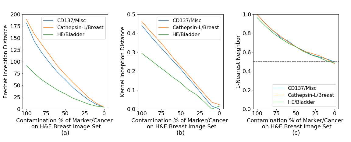
We used multiple cancer types and markers to account for alterations of color and shapes in the tissue. Markers highlight parts of the tissue with different colors, and cancer types have distinct tissues structures. Examples of these changes are displayed in Figure 33.

We constructed one reference image set with 5000 H&E breast cancer images from our data sets of NKI and VGH, and compared it against another set of 5000 H&E breast cancer images contaminated with other markers and cancer types. We used three types of marker-cancer combinations for contamination, all from the Stanford TMA Database (Marinelli et al., 2008): H&E - Bladder cancer, Cathepsin-L - Breast cancer, and CD137 - Lymph/Colon/Liver cancer.

Each set of images was constructed by randomly sampling from the respective marker-cancer type data set, which is done to minimize the overlap between the clean and contaminated sets.

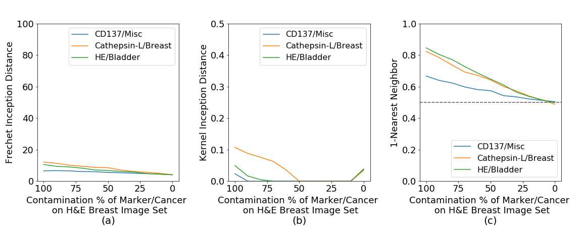
Figure 34 shows how (a) FID, (b) KID, (c) 1-NN behave when the reference H&E breast cancer set is measured against multiple percentage of contaminated H&E breast cancer sets. Marker types have a large impact due to color change and all metrics capture this except for 1-NN. Cathepsin-L highlights parts of the tissue with brown colors and CD137 has similar color to necrotic tissue on H&E breast cancer, but still far from the characteristic pink color of H&E. Accordingly, H&E-Bladder has a better score in all metrics due to the color stain, again expect for 1-NN. Cancer tissue type differences are captured by all the metrics, which shows a marker predominance, but we can see that on the H&E marker the differences between breast and bladder types are still captured.

In this experiment, we find that FID and KID have a gradual response distinguishing between markers and cancer tissue types, however 1-NN is not able to give a measure that clearly defines these changes.

I.2 Reliability on evaluation metrics

Another evaluation we performed was to study which metrics are consistent when two independent sample distributions with the same contamination percentage are compared. To construct this test, for each contamination percentage, we create two independent sample sets of 5000 images and compare them against each other. Again, we constructed these image sets by randomly selecting images for each of the marker-cancer databases. We do this to ensure there are no overlapping images between the distributions.

In Figure 35 we show that (a) FID has a stable performance, compared to (b) KID, and especially (c) 1-NN. The metrics should show a close to zero distance for each of the contamination rates since we are comparing two sample-distributions from the same data set. This shows that only FID has a close to zero constant behavior across different data sets when comparing the same tissue image distributions.

Based on these two experiments, we argue that 1-NN does not clearly represent changes in the cancer types and marker, and both KID and 1-NN do not give a constant reliable measure across different markers and cancer types. Therefore we focused on FID as the most promising evaluation metrics.

J Pathologists Tests

We provide in here examples of the tests taken by the pathologists:

Figure 36: Individual images for breast cancer tissue.

Figure 37: Individual images for colorectal cancer tissue.

K Model Architecture

Generator Network $G:w\rightarrow x$
Dense Layer, adaptive instance normalization (AdaIN), and leakyReLU
$200\rightarrow 1024$
Dense Layer, AdaIN, and leakyReLU
$1024\rightarrow 12544$
Reshape $7\times 7\times 256$
ResNet Conv2D Layer, 3x3, stride 1, pad same, AdaIN, and leakyReLU $0.2$
$7\times 7\times 256\rightarrow 7\times 7\times 256$
ConvTranspose2D Layer, 2x2, stride 2, pad upscale, AdaIN, and leakyReLU $0.2$
$7\times 7\times 256\rightarrow 14\times 14\times 512$
ResNet Conv2D Layer, 3x3, stride 1, pad same, AdaIN, and leakyReLU $0.2$
$14\times 14\times 512\rightarrow 14\times 14\times 512$
ConvTranspose2D Layer, 2x2, stride 2, pad upscale, AdaIN, and leakyReLU $0.2$
$14\times 14\times 512\rightarrow 28\times 28\times 256$
ResNet Conv2D Layer, 3x3, stride 1, pad same, AdaIN, and leakyReLU $0.2$
$28\times 28\times 256\rightarrow 28\times 28\times 256$
Attention Layer at $28\times 28\times 256$
ConvTranspose2D Layer, 2x2, stride 2, pad upscale, AdaIN, and leakyReLU $0.2$
$28\times 28\times 256\rightarrow 56\times 56\times 128$
ResNet Conv2D Layer, 3x3, stride 1, pad same, AdaIN, and leakyReLU $0.2$
$56\times 56\times 128\rightarrow 56\times 56\times 128$
ConvTranspose2D Layer, 2x2, stride 2, pad upscale, AdaIN, and leakyReLU $0.2$
$56\times 56\times 128\rightarrow 112\times 112\times 64$
ResNet Conv2D Layer, 3x3, stride 1, pad same, AdaIN, and leakyReLU $0.2$
$112\times 112\times 64\rightarrow 112\times 112\times 64$
ConvTranspose2D Layer, 2x2, stride 2, pad upscale, AdaIN, and leakyReLU $0.2$
$112\times 112\times 64\rightarrow 224\times 224\times 32$
Conv2D Layer, 3x3, stride 1, pad same, $32\rightarrow 3$
$224\times 224\times 32\rightarrow 224\times 224\times 3$
Sigmoid

Table 3: Generator Network Architecture details of PathologyGAN model.

Discriminator Network $C:x\rightarrow d$
$x\in\mathbb{R}^{224\times 224\times 3}$
ResNet Conv2D Layer, 3x3, stride 1, pad same, and leakyReLU $0.2$
$224\times 224\times 3\rightarrow 224\times 224\times 3$
Conv2D Layer, 2x2, stride 2, pad downscale, and leakyReLU $0.2$
$224\times 224\times 3\rightarrow 122\times 122\times 32$
ResNet Conv2D Layer, 3x3, stride 1, pad same, and leakyReLU $0.2$
$122\times 122\times 32\rightarrow 122\times 122\times 32$
Conv2D Layer, 2x2, stride 2, pad downscale, and leakyReLU $0.2$
$122\times 122\times 32\rightarrow 56\times 56\times 64$
ResNet Conv2D Layer, 3x3, stride 1, pad same, and leakyReLU $0.2$
$56\times 56\times 64\rightarrow 56\times 56\times 64$
Conv2D Layer, 2x2, stride 2, pad downscale, and leakyReLU $0.2$
$56\times 56\times 64\rightarrow 28\times 28\times 128$
ResNet Conv2D Layer, 3x3, stride 1, pad same, and leakyReLU $0.2$
$28\times 28\times 128\rightarrow 28\times 28\times 128$
Attention Layer at $28\times 28\times 128$
Conv2D Layer, 2x2, stride 2, pad downscale, and leakyReLU $0.2$
$28\times 28\times 128\rightarrow 14\times 14\times 256$
ResNet Conv2D Layer, 3x3, stride 1, pad same, and leakyReLU $0.2$
$14\times 14\times 256\rightarrow 14\times 14\times 256$
Conv2D Layer, 2x2, stride 2, pad downscale, and leakyReLU $0.2$
$14\times 14\times 256\rightarrow 7\times 7\times 512$
Flatten $7\times 7\times 512\rightarrow 25088$
Dense Layer and leakyReLU, $25088\rightarrow 1024$
Dense Layer and leakyReLU, $1024\rightarrow 1$

Table 4: Discriminator Network Architecture details of PathologyGAN model.

Mapping Network $M:z\rightarrow w$
$z\in\sim\mathbb{R}^{200}\sim\mathcal{N}(0,I)$
ResNet Dense Layer and ReLU, $200\rightarrow 200$
ResNet Dense Layer and ReLU, $200\rightarrow 200$
ResNet Dense Layer and ReLU, $200\rightarrow 200$
ResNet Dense Layer and ReLU, $200\rightarrow 200$
Dense Layer, $200\rightarrow 200$

Table 5: Mapping Network Architecture details of PathologyGAN model.

[bib.bib1] Barratt and Sharma (2018) Shane Barratt and Rishi Sharma. A note on the Inception score. CoRR, abs/1801.01973, 2018. URL http://arxiv.org/abs/1801.01973.

[bib.bib2] Beck et al. (2011) Andrew H Beck, Ankur R Sangoi, Samuel Leung, Robert J Marinelli, Torsten O Nielsen, Marc J van de Vijver, Robert B West, Matt van de Rijn, and Daphne Koller. Systematic analysis of breast cancer morphology uncovers stromal features associated with survival. Sci Transl Med, 3(108):108ra113, Nov 2011. ISSN 1946-6242 (Electronic); 1946-6234 (Linking). doi: 10.1126/scitranslmed.3002564.

[bib.bib3] Bergenstråhle et al. (2020a) Joseph Bergenstråhle, Ludvig Larsson, and Joakim Lundeberg. Seamless integration of image and molecular analysis for spatial transcriptomics workflows. BMC Genomics, 21(1):482, 2020a. doi: 10.1186/s12864-020-06832-3. URL https://doi.org/10.1186/s12864-020-06832-3.

[bib.bib4] Bergenstråhle et al. (2020b) Ludvig Bergenstråhle, Bryan He, Joseph Bergenstråhle, Alma Andersson, Joakim Lundeberg, James Zou, and Jonas Maaskola. Super-resolved spatial transcriptomics by deep data fusion. bioRxiv, page 2020.02.28.963413, 01 2020b.

[bib.bib5] Bińkowski et al. (2018) Mikołaj Bińkowski, Dougal J. Sutherland, Michael Arbel, and Arthur Gretton. Demystifying MMD GANs. In International Conference on Learning Representations, 2018. URL https://openreview.net/forum?id=r1lUOzWCW.

[bib.bib6] Brock et al. (2019) Andrew Brock, Jeff Donahue, and Karen Simonyan. Large scale GAN training for high fidelity natural image synthesis. In International Conference on Learning Representations, 2019. URL https://openreview.net/forum?id=B1xsqj09Fm.

[bib.bib7] Campbell et al. (2020) Peter J. Campbell, Gad Getz, Jan O. Korbel, and et al. Pan-cancer analysis of whole genomes. Nature, 578(7793):82–93, 2020.

[bib.bib8] Coudray and Tsirigos (2020) Nicolas Coudray and Aristotelis Tsirigos. Deep learning links histology, molecular signatures and prognosis in cancer. Nature Cancer, 1(8):755–757, 2020. doi: 10.1038/s43018-020-0099-2. URL https://doi.org/10.1038/s43018-020-0099-2.

[bib.bib9] Coudray et al. (2018) Nicolas Coudray, Paolo Santiago Ocampo, Theodore Sakellaropoulos, Navneet Narula, Matija Snuderl, David Fenyö, Andre L. Moreira, Narges Razavian, and Aristotelis Tsirigos. Classification and mutation prediction from non–small cell lung cancer histopathology images using deep learning. Nature Medicine, 24(10):1559–1567, 2018. doi: 10.1038/s41591-018-0177-5. URL https://doi.org/10.1038/s41591-018-0177-5.

[bib.bib10] de Bel et al. (2018) Thomas de Bel, Meyke Hermsen, Bart Smeets, Luuk Hilbrands, Jeroen van der Laak, and Geert Litjens. Automatic segmentation of histopathological slides of renal tissue using deep learning. In Medical Imaging 2018: Digital Pathology, volume 10581, page 1058112. International Society for Optics and Photonics, 2018.

[bib.bib11] Deng et al. (2009) J. Deng, W. Dong, R. Socher, L.-J. Li, K. Li, and L. Fei-Fei. ImageNet: A Large-Scale Hierarchical Image Database. In CVPR09, 2009.

[bib.bib12] Dentro et al. (2020) Stefan C. Dentro, Ignaty Leshchiner, and et al. Characterizing genetic intra-tumor heterogeneity across 2,658 human cancer genomes. bioRxiv, 2020. doi: 10.1101/312041. URL https://www.biorxiv.org/content/early/2020/04/22/312041.

[bib.bib13] Fréchet (1957) Maurice Fréchet. Sur la distance de deux lois de probabilité. COMPTES RENDUS HEBDOMADAIRES DES SEANCES DE L ACADEMIE DES SCIENCES, 244(6):689–692, 1957.

[bib.bib14] Fu et al. (2020) Yu Fu, Alexander W. Jung, Ramon Viñas Torne, Santiago Gonzalez, Harald Vöhringer, Artem Shmatko, Lucy R. Yates, Mercedes Jimenez-Linan, Luiza Moore, and Moritz Gerstung. Pan-cancer computational histopathology reveals mutations, tumor composition and prognosis. Nature Cancer, 1(8):800–810, 2020. doi: 10.1038/s43018-020-0085-8. URL https://doi.org/10.1038/s43018-020-0085-8.

[bib.bib15] Gadermayr et al. (2018) Michael Gadermayr, Laxmi Gupta, Barbara M Klinkhammer, Peter Boor, and Dorit Merhof. Unsupervisedly training gans for segmenting digital pathology with automatically generated annotations. arXiv preprint arXiv:1805.10059, 2018.

[bib.bib16] Gadermayr et al. (2019) Michael Gadermayr, Laxmi Gupta, Vitus Appel, Peter Boor, Barbara M Klinkhammer, and Dorit Merhof. Generative adversarial networks for facilitating stain-independent supervised and unsupervised segmentation: a study on kidney histology. IEEE transactions on medical imaging, 38(10):2293–2302, 2019.

[bib.bib17] Gerstung et al. (2020) Moritz Gerstung, Clemency Jolly, and et al. The evolutionary history of 2,658 cancers. Nature, 578(7793):122–128, 2020.

[bib.bib18] Goodfellow et al. (2014) Ian Goodfellow, Jean Pouget-Abadie, Mehdi Mirza, Bing Xu, David Warde-Farley, Sherjil Ozair, Aaron Courville, and Yoshua Bengio. Generative adversarial nets. In Z. Ghahramani, M. Welling, C. Cortes, N. D. Lawrence, and K. Q. Weinberger, editors, Advances in Neural Information Processing Systems 27, pages 2672–2680. Curran Associates, Inc., 2014. URL http://papers.nips.cc/paper/5423-generative-adversarial-nets.pdf.

[bib.bib19] Gretton et al. (2012) Arthur Gretton, Karsten M. Borgwardt, Malte J. Rasch, Bernhard Schölkopf, and Alexander Smola. A kernel two-sample test. Journal of Machine Learning Research, 13(25):723–773, 2012. URL http://jmlr.org/papers/v13/gretton12a.html.

[bib.bib20] He et al. (2020) Bryan He, Ludvig Bergenstråhle, Linnea Stenbeck, Abubakar Abid, Alma Andersson, Åke Borg, Jonas Maaskola, Joakim Lundeberg, and James Zou. Integrating spatial gene expression and breast tumour morphology via deep learning. Nature Biomedical Engineering, 4(8):827–834, 2020. doi: 10.1038/s41551-020-0578-x. URL https://doi.org/10.1038/s41551-020-0578-x.

[bib.bib21] He et al. (2016) Kaiming He, Xiangyu Zhang, Shaoqing Ren, and Jian Sun. Deep residual learning for image recognition. 2016 IEEE Conference on Computer Vision and Pattern Recognition (CVPR), Jun 2016. doi: 10.1109/cvpr.2016.90. URL http://dx.doi.org/10.1109/cvpr.2016.90.

[bib.bib22] Heusel et al. (2017) Martin Heusel, Hubert Ramsauer, Thomas Unterthiner, Bernhard Nessler, and Sepp Hochreiter. Gans trained by a two time-scale update rule converge to a local nash equilibrium. In I. Guyon, U. V. Luxburg, S. Bengio, H. Wallach, R. Fergus, S. Vishwanathan, and R. Garnett, editors, Advances in Neural Information Processing Systems 30, pages 6626–6637. Curran Associates, Inc., 2017.

[bib.bib23] Hou et al. (2019) Le Hou, Vu Nguyen, Ariel B Kanevsky, Dimitris Samaras, Tahsin M Kurc, Tianhao Zhao, Rajarsi R Gupta, Yi Gao, Wenjin Chen, David Foran, and Joel H Saltz. Sparse autoencoder for unsupervised nucleus detection and representation in histopathology images. Pattern recognition, 86:188–200, 02 2019. doi: 10.1016/j.patcog.2018.09.007. URL https://pubmed.ncbi.nlm.nih.gov/30631215.

[bib.bib24] Hu et al. (2019) Bo Hu, Ye Tang, Eric I-Chao Chang, Yubo Fan, Maode Lai, and Yan Xu. Unsupervised learning for cell-level visual representation in histopathology images with generative adversarial networks. IEEE Journal of Biomedical and Health Informatics, 23(3):1316–1328, May 2019. ISSN 2168-2208. doi: 10.1109/jbhi.2018.2852639. URL http://dx.doi.org/10.1109/JBHI.2018.2852639.

[bib.bib25] Huang et al. (2018) Gao Huang, Yang Yuan, Qiantong Xu, Chuan Guo, Yu Sun, Felix Wu, and Kilian Weinberger. An empirical study on evaluation metrics of generative adversarial networks, 2018. URL https://openreview.net/forum?id=Sy1f0e-R-.

[bib.bib26] Jolicoeur-Martineau (2019) Alexia Jolicoeur-Martineau. The relativistic discriminator: a key element missing from standard GAN. In International Conference on Learning Representations, 2019. URL https://openreview.net/forum?id=S1erHoR5t7.

[bib.bib27] Karras et al. (2019) Tero Karras, Samuli Laine, and Timo Aila. A style-based generator architecture for generative adversarial networks. 2019 IEEE/CVF Conference on Computer Vision and Pattern Recognition (CVPR), Jun 2019. doi: 10.1109/cvpr.2019.00453. URL http://dx.doi.org/10.1109/CVPR.2019.00453.

[bib.bib28] Kather et al. (2018) Jakob Nikolas Kather, Niels Halama, and Alexander Marx. 100,000 histological images of human colorectal cancer and healthy tissue, April 2018. URL https://doi.org/10.5281/zenodo.1214456.

[bib.bib29] Kather et al. (2020) Jakob Nikolas Kather, Lara R. Heij, Heike I. Grabsch, and et al. Pan-cancer image-based detection of clinically actionable genetic alterations. Nature Cancer, 1(8):789–799, 2020. doi: 10.1038/s43018-020-0087-6. URL https://doi.org/10.1038/s43018-020-0087-6.

[bib.bib30] Katzman et al. (2018) Jared L. Katzman, Uri Shaham, Alexander Cloninger, Jonathan Bates, Tingting Jiang, and Yuval Kluger. Deepsurv: personalized treatment recommender system using a cox proportional hazards deep neural network. BMC Medical Research Methodology, 18(1), Feb 2018. ISSN 1471-2288. doi: 10.1186/s12874-018-0482-1. URL http://dx.doi.org/10.1186/s12874-018-0482-1.

[bib.bib31] Kingma and Ba (2014) Diederik P Kingma and Jimmy Ba. Adam: A method for stochastic optimization. arXiv preprint arXiv:1412.6980, 2014.

[bib.bib32] Lee et al. (2018) C. Lee, W. Zame, Jinsung Yoon, and M. V. D. Schaar. Deephit: A deep learning approach to survival analysis with competing risks. In AAAI, 2018.

[bib.bib33] Levine et al. (2020) Adrian B Levine, Jason Peng, David Farnell, Mitchell Nursey, and et al. Synthesis of diagnostic quality cancer pathology images by generative adversarial networks. The Journal of Pathology, 252(2):178–188, 2020. doi: https://doi.org/10.1002/path.5509. URL https://onlinelibrary.wiley.com/doi/abs/10.1002/path.5509.

[bib.bib34] Lim and Ye (2017) Jae Hyun Lim and Jong Chul Ye. Geometric GAN, 2017.

[bib.bib35] Lopez-Paz and Oquab (2016) David Lopez-Paz and Maxime Oquab. Revisiting classifier two-sample tests, 2016.

[bib.bib36] Mahmood et al. (2018) Faisal Mahmood, Daniel Borders, Richard Chen, Gregory McKay, Kevan J Salimian, Alexander Baras, and Nicholas Durr. Deep adversarial training for multi-organ nuclei segmentation in histopathology images, 09 2018.

[bib.bib37] Marinelli et al. (2008) Robert J. Marinelli, Kelli Montgomery, Chih Long Liu, Nigam Shah, Wijan Prapong, Michael Nitzberg, Zachariah K Zachariah, Gavin Sherlock, Yasodha Natkunam, Robert B West, Matt van de Rijn, Patrick O Brown, and Catherine A Ball. The stanford tissue microarray database. Nucleic acids research, 36:D871–7, 02 2008. doi: 10.1093/nar/gkm861.

[bib.bib38] McInnes et al. (2018) Leland McInnes, John Healy, Nathaniel Saul, and Lukas Großberger. UMAP: Uniform Manifold Approximation and Projection. Journal of Open Source Software, 3(29), 2018.

[bib.bib39] Miyato et al. (2018) Takeru Miyato, Toshiki Kataoka, Masanori Koyama, and Yuichi Yoshida. Spectral normalization for generative adversarial networks. In International Conference on Learning Representations, 2018. URL https://openreview.net/forum?id=B1QRgziT-.

[bib.bib40] Qaiser et al. (2019) Talha Qaiser, Yee-Wah Tsang, Daiki Taniyama, Naoya Sakamoto, Kazuaki Nakane, David Epstein, and Nasir Rajpoot. Fast and accurate tumor segmentation of histology images using persistent homology and deep convolutional features. Medical image analysis, 55:1–14, 2019.

[bib.bib41] Qu et al. (2019) Hui Qu, Gregory Riedlinger, Pengxiang Wu, Qiaoying Huang, Jingru Yi, Subhajyoti De, and Dimitris Metaxas. Joint segmentation and fine-grained classification of nuclei in histopathology images. In 2019 IEEE 16th International Symposium on Biomedical Imaging (ISBI 2019), pages 900–904. IEEE, 2019.

[bib.bib42] Quiros et al. (2020) Adalberto Claudio Quiros, Roderick Murray-Smith, and Ke YuCoudan. Learning a low dimensional manifold of real cancer tissue with pathologygan, 2020.

[bib.bib43] Radford et al. (2015) Alec Radford, Luke Metz, and Soumith Chintala. Unsupervised representation learning with deep convolutional generative adversarial networks, 2015.

[bib.bib44] Rana et al. (2018) Aman Rana, Gregory Yauney, Alarice Lowe, and Pratik Shah. Computational histological staining and destaining of prostate core biopsy RGB images with Generative Adversarial Neural Networks. 2018 17th IEEE International Conference on Machine Learning and Applications (ICMLA), Dec 2018. doi: 10.1109/icmla.2018.00133. URL http://dx.doi.org/10.1109/ICMLA.2018.00133.

[bib.bib45] Salimans et al. (2016) Tim Salimans, Ian Goodfellow, Wojciech Zaremba, Vicki Cheung, Alec Radford, Xi Chen, and Xi Chen. Improved techniques for training gans. In D. D. Lee, M. Sugiyama, U. V. Luxburg, I. Guyon, and R. Garnett, editors, Advances in Neural Information Processing Systems 29, pages 2234–2242. Curran Associates, Inc., 2016. URL http://papers.nips.cc/paper/6125-improved-techniques-for-training-gans.pdf.

[bib.bib46] Schmauch et al. (2020) Benoît Schmauch, Alberto Romagnoni, Elodie Pronier, Charlie Saillard, Pascale Maillé, Julien Calderaro, Aurélie Kamoun, Meriem Sefta, Sylvain Toldo, Mikhail Zaslavskiy, Thomas Clozel, Matahi Moarii, Pierre Courtiol, and Gilles Wainrib. A deep learning model to predict rna-seq expression of tumours from whole slide images. Nature Communications, 11(1):3877, 2020. doi: 10.1038/s41467-020-17678-4. URL https://doi.org/10.1038/s41467-020-17678-4.

[bib.bib47] Szegedy et al. (2016) C. Szegedy, V. Vanhoucke, S. Ioffe, J. Shlens, and Z. Wojna. Rethinking the inception architecture for computer vision. In 2016 IEEE Conference on Computer Vision and Pattern Recognition (CVPR), pages 2818–2826, 2016. doi: 10.1109/CVPR.2016.308.

[bib.bib48] Tellez et al. (2018) David Tellez, Maschenka Balkenhol, Irene Otte-Höller, Rob van de Loo, Rob Vogels, Peter Bult, Carla Wauters, Willem Vreuls, Suzanne Mol, Nico Karssemeijer, et al. Whole-slide mitosis detection in h&e breast histology using phh3 as a reference to train distilled stain-invariant convolutional networks. IEEE transactions on medical imaging, 37(9):2126–2136, 2018.

[bib.bib49] Vickovic et al. (2019) Sanja Vickovic, Gökcen Eraslan, Fredrik Salmén, and et al. High-definition spatial transcriptomics for in situ tissue profiling. Nature Methods, 16(10):987–990, 2019.

[bib.bib50] Wang et al. (2020) Yuliang Wang, Shuyi Ma, and Walter L. Ruzzo. Spatial modeling of prostate cancer metabolic gene expression reveals extensive heterogeneity and selective vulnerabilities. Scientific Reports, 10(1):3490, 2020. doi: 10.1038/s41598-020-60384-w. URL https://doi.org/10.1038/s41598-020-60384-w.

[bib.bib51] Wei et al. (2019) Jason W. Wei, Laura J. Tafe, Yevgeniy A. Linnik, Louis J. Vaickus, Naofumi Tomita, and Saeed Hassanpour. Pathologist-level classification of histologic patterns on resected lung adenocarcinoma slides with deep neural networks. Scientific Reports, 9(1):3358, 2019. doi: 10.1038/s41598-019-40041-7. URL https://doi.org/10.1038/s41598-019-40041-7.

[bib.bib52] Woerl et al. (2020) Ann-Christin Woerl, Markus Eckstein, Josephine Geiger, Daniel C. Wagner, Tamas Daher, Philipp Stenzel, Aurélie Fernandez, Arndt Hartmann, Michael Wand, Wilfried Roth, and Sebastian Foersch. Deep learning predicts molecular subtype of muscle-invasive bladder cancer from conventional histopathological slides. European Urology, 78(2):256 – 264, 2020. ISSN 0302-2838. doi: https://doi.org/10.1016/j.eururo.2020.04.023. URL http://www.sciencedirect.com/science/article/pii/S0302283820302554.

[bib.bib53] Xu et al. (2019a) Bolei Xu, Jingxin Liu, Xianxu Hou, Bozhi Liu, Jon Garibaldi, Ian O Ellis, Andy Green, Linlin Shen, and Guoping Qiu. Look, investigate, and classify: A deep hybrid attention method for breast cancer classification. In 2019 IEEE 16th international symposium on biomedical imaging (ISBI 2019), pages 914–918. IEEE, 2019a.

[bib.bib54] Xu et al. (2016) Jun Xu, Lei Xiang, Qingshan Liu, Hannah Gilmore, Jianzhong Wu, Jinghai Tang, and Anant Madabhushi. Stacked sparse autoencoder (ssae) for nuclei detection on breast cancer histopathology images. IEEE transactions on medical imaging, 35(1):119–130, 01 2016. doi: 10.1109/TMI.2015.2458702. URL https://pubmed.ncbi.nlm.nih.gov/26208307.

[bib.bib55] Xu et al. (2018) Qiantong Xu, Gao Huang, Yang Yuan, Chuan Guo, Yu Sun, Felix Wu, and Kilian Q. Weinberger. An empirical study on evaluation metrics of generative adversarial networks. CoRR, abs/1806.07755, 2018. URL http://arxiv.org/abs/1806.07755.