

1 Introduction
Learning-based medical image analysis has become widespread with the advent of deep learning. However, most deep learning models rely on large pools of labeled data. Especially in the medical imaging domain, obtaining copious labeled imagery is often infeasible, as annotation requires substantial domain expertise and manual labor. Therefore, developing large-scale deep learning methodologies for medical image analysis tasks is challenging. In confronting the limited labeled data problem, Semi-Supervised Learning (SSL) has been gaining attention. In semi-supervised learning, unlabeled training examples are leveraged in combination with labeled examples to maximize information gains (Chapelle et al., 2009). Specifically within the medical domain, where collecting data is generally easier than annotating those data, the use of deep learning for medical image analysis tasks can be fostered by leveraging semi-supervised learning.
Recent research has yielded a variety of semi-supervised learning techniques (Imran, 2020). Pseudo-labeling (Lee, 2013) trains a model with labeled data and unlabeled data simultaneously, generating labels for the unlabeled data by assuming the model-predicted labels to be reliable. Similarly, entropy minimization (Grandvalet and Bengio, 2005) trains so as to match the predicted data distribution of unlabeled data with that of the labeled data, under the assumption that unlabeled examples should yield prediction distributions that are similar to those from labeled examples (Ouali et al., 2020). Domain adaptation (Beijbom, 2012) is a form of inductive transfer learning, where a model is trained on labeled data from the source domain as well as labeled plus unlabeled data from the target domain, which improves model generalization for the target domain, but lacks clinical value if the target domain data is inaccessible during training.
Thus, progress has been made in learning from limited labeled data, although mainly within the confines of single-task learning. In particular, individual medical imaging tasks, such as diagnostic classification and anatomical segmentation, have been addressed using state-of-the-art Convolutional Neural Network (CNN) models (Anwar et al., 2018); e.g., for medical image segmentation, encoder-decoder networks (Ronneberger et al., 2015), variational auto-encoder networks, (Myronenko, 2018), context encoder networks (Gu et al., 2019), multiscale adversarial learning (Imran and Terzopoulos, 2021a), etc.
By contrast, Multi-Task Learning (MTL) is defined as optimizing more than one loss in a single model such that multiple related tasks are performed by sharing the learned representation (Ruder, 2017). Jointly training multiple tasks within a model improves the generalizability of the model as each of the tasks regularizes the others (Caruana, 1993). Assuming that training data with limited annotations come from different distributions for different tasks, multi-task learning may be useful in such scenarios for learning in a scarcely-supervised manner (Imran et al., 2020; Imran and Terzopoulos, 2021b).
Combining the objectives of substantially unlabeled data training and multi-task learning, Semi-Supervised Multi-Task Learning (SSMTL) is a promising research area in the context of medical image analysis. While there have been prior efforts on multi-tasking (Mehta et al., 2018; Girard et al., 2019), rarely do they focus on incorporating semi-supervised learning particularly within the medical realm. Liu et al. (2008) proposed a general semi-supervised multi-tasking method that uses soft-parameter sharing to allow multiple classification tasks in a single model. Gao et al. (2019) performed multi-tasking on tasks within the same medical domain by exploiting feature transfer. Adversarial learning (Salimans et al., 2016) combines a classifier with a discriminator to perform semi-supervised, adversarial multi-tasking. Imran and Terzopoulos (2019) introduced semi-supervised multi-task learning using adversarial learning and attention masking. Zhou et al. (2019) proposed a semi-supervised multi-tasking model that uses an attention mechanism to grade segmented retinal images. None of the aforecited works, however, take into consideration the disparity in the training data distributions for multiple tasks.
To learn diagnostic classification and anatomical segmentation jointly from substantially unlabeled multi-source data, we propose MultiMix, a novel, better-generalized multi-tasking model that incorporates confidence-based augmentation and a module that bridges the classification and segmentation tasks. This saliency bridge module produces a saliency map by computing the gradient of the class score with respect to the input image, thus not only enabling the analysis of the model’s predictions, but also improving the model’s performance of both tasks. While the explainability of any deep learning model can be based on visualizing saliency maps (Simonyan et al., 2014; Zhang et al., 2016; Hu et al., 2019), to our knowledge a saliency bridge between two shared tasks within a single model has not previously been explored. We demonstrate that the saliency bridge module in conjunction with a simple yet effective semi-supervised learning method in a multi-tasking setting can yield improved and consistent performance across multiple domains.
This article is a revised and extended version of our ISBI publication (Haque et al., 2021).111With an augmented literature review, a more detailed explanation of the methods, model architecture, and training algorithm, further details about the datasets, saliency map visualizations from multiple datasets, and additional results and discussion supported by quantitative (performance metrics tables) and qualitative (mask predictions, Bland Altman plots, ROC curves, consistency plots) characteristics. Our main contributions may be summarized as follows:
- •
A new semi-supervised learning model, MultiMix, that exploits confidence-based data augmentation and consistency regularization to jointly learn diagnostic classification and anatomical segmentation from multi-source, multi-domain medical image datasets.
- •
Incorporation of an innovative saliency bridge module connecting the segmentation and classification branches of the model, resulting in the improved performance of both tasks.
- •
Substantiation of the improved generalizability (both in-domain and cross-domain) of the proposed model via experimentation with varied quantities of labeled data and mixed data sources related to multiple tasks, specifically in the classification of pneumonia and the simultaneous segmentation of the lungs in chest X-ray images.
- •
MultiMix software made available at https://github.com/ayaanzhaque/MultiMix.
2 The MultiMix Model
To formulate our approach, we assume unknown data distributions over images and class labels as well as over images and segmentation labels . Hence, segmentation labels for the images and class labels for the images are unavailable. We also assume access to labeled training sets sampled i.i.d. from and sampled i.i.d. from , along with unlabeled training sets sampled i.i.d. from and sampled i.i.d. from , after marginalizing out and , respectively.
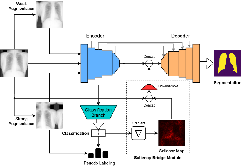
In our MultiMix model (Figure 1), we utilize a U-Net-like (Ronneberger et al., 2015) encoder-decoder architecture for image deconstruction and reconstruction. The encoder functions similarly to a standard CNN. To perform multi-tasking, we use pooling layers followed by fully-connected layers, allowing the encoder to output class predictions through the classification branch of the model. Furthermore, in the segmentaton branch of the model, the segmentation predictions are obtained as the output of the decoder.
MultiMix performs multi-tasking in a semi-supervised learning manner, assuming the training data for the two tasks come from disparate distributions. It is well established that a multi-tasking model usually outperforms its single-task counterparts (Imran and Terzopoulos, 2019; Imran et al., 2020; Imran, 2020). The shared encoder in the MultiMix model learns features useful for addressing both the classification and segmentation tasks. This joint representation learning enables the model to avoid overfitting and generalize better. Most importantly, it exploits the relatedness of the tasks, which is crucial for effective multi-tasking.
In the following sections, we describe the classification and segmentation branches of the MultiMix model, explain the saliency bridge module that bridges the two branches, and specify the MultiMix training procedure.
2.1 Classification Branch
For semi-supervised classification, we leverage data augmentation and pseudo-labeling. Inspired by the work of Sohn et al. (2020), for each unlabeled image we perform two degrees of augmentation: weak and strong. The former consists of standard augmentations—both random horizontal flipping and random cropping—and is applied to the labeled data as well, whereas the latter is performed by randomly applying any number of augmentations from a pool of “heavy” augmentations.222This pool includes augmentations such as horizontal flip, crop, autocontrast, brightness, contrast, equalize, identity, posterize, rotate, sharpness, shearX, shearY, solarize, translateX, and TranslateY. Autocontrast, brightness, contrast, and equalize are all severe image intensity modifications. An unlabeled image is first weakly augmented, , and a pseudo-label is synthesized from using the model prediction . The image-label pair is retained only if the confidence with which the model generates the pseudo-label exceeds the experimentally tuned threshold , thus deterring learning from poor and incorrect labels. Second, are strongly augmented versions of .
Our training strategy promotes effective learning from large amounts of unlabeled data, which is challenging. At first, the predictions are less reliable as the model begins to learn mainly from the labeled data, but the model gains confidence with the generation of labels for the unlabeled images and, as a result, it becomes more proficient. Since the unlabeled examples are incrementally added to the training set, subject to the threshold, the model learns to predict more accurately in a progressive manner and, with increasing confidence, the performance of the model improves at an increasingly higher rate. Furthermore, employing two degrees of augmentation enables the model to maximize its knowledge gain from the unlabeled data due to the enhanced image diversity through what is known as consistency learning as, in theory, two augmented versions of the same image should yield the same prediction, which is encouraged using an unsupervised loss. In other words, imposing on the model, through an unsupervised loss, to produce the same predictions on images subjected to two different degrees of augmentation results in better classification performance.
The classification objective
| (1) |
includes a supervised loss component for the labeled data, which uses cross-entropy between the reference class label and the model prediction , as well as an unsupervised loss component for the unlabeled data, which uses cross-entropy between the pseudo-label and the model prediction .
Note that the model is trained to ignore GAug as it is provided the pseudo-label . Since the underlying data distributions are the same for both augmentations, it is compelled to learn that for the sake of consistency. Weak augmentations are used to produce reliable and usable pseudo-labels whereas strong augmentations are used to provide a difficult challenge for the model. This difficulty forces the model to learn more effective representations in order to be accurate, and it also prevents overfitting from minimizing the loss too early. With the assumption that the weakly augmented image has the correct label to be associated with the strongly augmented image, the model is empowered to discern the augmentations in the image, and its performance improves as a result, by learning the underlying features crucial to the diagnosis. This helps achieve better generalization despite the differences in data distributions across different domains. By teaching the model to learn only the more salient representations that will exist to some extent in all domains, it can generalize and be effective across domains.
2.2 Segmentation Branch
For segmentation, the predictions are made through the encoder-decoder architecture with skip connections. For the labeled samples , we calculate the direct segmentation loss in the form of Dice loss between the reference lung mask and predicted segmentation . Since we do not have the segmentation masks for the unlabeled examples , we cannot directly calculate the segmentation loss for them. To ensure consistency, we compute the KL divergence between segmentation predictions for the labeled examples and unlabeled examples . This penalizes the model for making predictions that increasingly differ from those of the labeled data, which helps the model fit the unlabeled data. The total segmentation objective is therefore
| (2) |
where and are weights.
2.3 Saliency Bridge Module
We incorporate a saliency bridge module to bridge between the classification and segmentation branches of the MultiMix model, as indicated in Figure 1. To learn which image regions are most relevant to classification, saliency maps
| (3) |
where and denote the class predictions for the input images and , respectively, are generated from the classification branch by computing the gradient of the predicted class with respect to the input image.333These saliency maps should not be confused with simultaneous segmentation and saliency detection or prediction, where a semantic segmentation model is trained to produce saliency maps to accompany the output segmentation masks; e.g., (Zeng et al., 2019). Our saliency bridge module is novel in that it performs a saliency analysis of MultiMix’s classification branch and leverages it to improve the performance of its semantic segmentation branch. It cannot be directly known if the image samples in represent normal or diseased cases, thus and are considered to be unlabeled for the classification task. Therefore, the saliency maps generated via the class prediction are not true segmentation maps, but they will nonetheless highlight the lungs or lung regions relevant to the particular disease class (see Appendix C).
The outputs of the saliency bridge module,
| (4) |
obtained by concatenating the saliency maps with the associated input images, are further downsampled before they are concatenated with the encoder-decoder bottleneck in the segmentation branch. This results in a tighter connection between the classification and segmentation tasks and improves the effectiveness of the bridge module, which retains important information from the encoder that may otherwise be lost because of the repeated convolutions. The saliency maps serve to guide the segmentation during the decoding phase, yielding improved segmentation while learning from limited labeled data. With improving classification performance, the saliency maps become more accurate, thus yielding improved segmentations, since the shared parameters responsible for improved classification produce a feedback loop that allows both tasks to improve jointly.
Conventionally, saliency maps are used to analyze which features and areas of the image are most relevant for classification, thereby enhancing understanding of the model’s learning process. Similarly, our saliency module is explainable, as it is a relevant connection between the classification and segmentation tasks (although model explainability in and of itself is not the main focus of our work). Since the saliency maps are comparable to segmentation masks, it is sensible to employ them to guide the decoder in the task of segmentation. Multi-tasking requires the tasks to be somewhat related, so our task-relevant bridge fosters a tighter bond between classification and segmentation.
2.4 MultiMix Training Procedure
Algorithm 1 presents the main steps of the MultiMix training procedure applied to labeled and unlabeled classification and segmentation training data. The model is trained simultaneously on the classification objective (1) and segmentation objective (2) using the following total loss for a minibatch size of :
| (5) |
3 Experimental Evaluation
3.1 Data
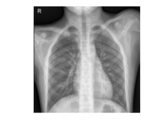
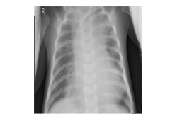
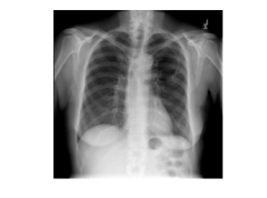
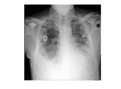
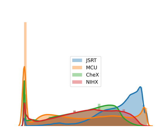
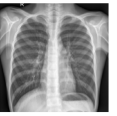
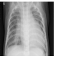
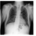
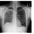
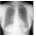
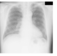
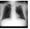
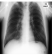
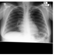
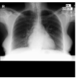
Models were trained and tested in the combined classification and segmentation tasks using chest X-ray images from two different sources: pneumonia detection (CheX) (Kermany et al., 2018) and the Japanese Society of Radiological Technology (JSRT) (Shiraishi et al., 2000). We further validated the models using the Montgomery County chest X-rays (MCU) (Jaeger et al., 2014) and a subset of the NIH chest X-ray dataset (NIHX) (Wang et al., 2017) (Figure 2(a)). Table 1 presents some details about the datasets used in our experiments. In addition to the diversity in the source, image quality, size, and proportion of normal and abnormal images, the disparity in the intensity distributions of the four datasets is also evident (Figure 2(b)). All the images were normalized and resized to before passing them to the models.
| Normal | Abnormal |
| CheX | |
 |  |
| NIHX | |
 |  |
| Mode | Dataset | Total | Normal | Abnormal | Train | Val | Test | |||
|---|---|---|---|---|---|---|---|---|---|---|
| in-domain | JSRT | 247 | – | – | 111 | 13 | 123 | |||
| CheX | 5,856 | 1583 | 4273 | 5216 | 16 | 624 | ||||
| cross-domain | MCU | 138 | – | – | 93 | 10 | 35 | |||
| NIHX | 4185 | 2754 | 1431 | – | – | 4185 |
3.2 Implementation Details
Baselines:
We used the U-Net and encoder-only (Enc) networks separately for the single-task baseline models in both the fully supervised and semi-supervised schemes. Using the same backbone network, we also trained a multi-tasking U-Net with the classification branch (UMTL). All these models incorporate an INorm, LReLU, and dropout at every convolutional block (see Appendix A). Moreover, we performed ablation experiments to assess the impact of each key piece of our MultiMix model: single-task Enc-SSL (encoder with confidence-based augmentation SSL), single-task Enc-MM (an implementation of MixMatch (Berthelot et al., 2019)), UMTL-S (UMTL with saliency bridge), UMTL-SSL (UMTL with SSL classification), and UMTL-SSL-S (UMTL with saliency bridge and confidence-based augmentation).
Augmentations:
We performed random horizontal flip and crop in WAug for the examples in . On the other hand, GAug was applied through a random combination from the pool of augmentations: random horizontal flip, crop (), autocontrast, brightness, contrast, equalize, identity, posterize, rotate (), sharpness, shearX, shearY, solarize, translateX (30%), and translateY (30%).
Training:
All the models (single-task or multi-task) were trained on varying (10, 50, full), and (100, 1000, full). Each experiment was repeated 5 times and the average performance is reported. We implemented the models using Python and the PyTorch framework and trained using an Nvidia K80 GPU.
Hyper-parameters:
We used the Adam optimizer with adaptive learning rates of 0.1 every 8 epochs and an initial learning rate of 0.0001. A negative slope of 0.2 was applied to Leaky ReLU, and the dropout was set to 0.25. We set , , (for smaller ) and . Each model was trained with a mini-batch size of . All model-specific hyperparameters were experimentally tuned. We found that the performance of the model varied only minimally subject to the different choices.
Evaluation:
For classification, along with the overall accuracy (Acc), we recorded the class-wise F1 scores (F1-N for normal and F1-P for pneumonia). To evaluate segmentation performance, we used the Dice similarity (DS), Jaccard similarity (JS), structural similarity measure (SSIM), average Hausdorff distance (HD), precision (P), and Recall (R) scores.
| Model | Classification | Segmentation | |||||||||||||
| Acc | F1-Nor | F1-Abn | DS | JS | SSIM | HD | P | R | |||||||
| U-Net | — | — | — | — | 10 | ||||||||||
| — | — | — | — | 50 | |||||||||||
| — | — | — | — | Full | |||||||||||
| Enc | 100 | — | — | — | — | — | — | — | |||||||
| 1000 | — | — | — | — | — | — | — | ||||||||
| Full | — | — | — | — | — | — | — | ||||||||
| Enc-MM | 100 | — | — | — | — | — | — | — | |||||||
| 1000 | — | — | — | — | — | — | — | ||||||||
| Full | — | — | — | — | — | — | — | ||||||||
| Enc-SSL | 100 | — | — | — | — | — | — | — | |||||||
| 1000 | — | — | — | — | — | — | — | ||||||||
| Full | — | — | — | — | — | — | — | ||||||||
| UMTL | 100 | 10 | |||||||||||||
| 100 | 50 | ||||||||||||||
| 100 | Full | ||||||||||||||
| 1000 | 10 | ||||||||||||||
| 1000 | 50 | ||||||||||||||
| 1000 | Full | ||||||||||||||
| Full | 10 | ||||||||||||||
| Full | 50 | ||||||||||||||
| Full | Full | ||||||||||||||
| UMTL-S | 100 | 10 | |||||||||||||
| 100 | 50 | ||||||||||||||
| 100 | Full | ||||||||||||||
| 1000 | 10 | ||||||||||||||
| 1000 | 50 | ||||||||||||||
| 1000 | Full | ||||||||||||||
| Full | 10 | ||||||||||||||
| Full | 50 | ||||||||||||||
| Full | Full | ||||||||||||||
| UMTL-SSL | 100 | 10 | |||||||||||||
| 100 | 50 | ||||||||||||||
| 100 | Full | ||||||||||||||
| 1000 | 10 | ||||||||||||||
| 1000 | 50 | ||||||||||||||
| 1000 | Full | ||||||||||||||
| Full | 10 | ||||||||||||||
| Full | 50 | ||||||||||||||
| Full | Full | ||||||||||||||
| UMTL-SSL-S | 100 | 10 | |||||||||||||
| 100 | 50 | ||||||||||||||
| 100 | Full | ||||||||||||||
| 1000 | 10 | ||||||||||||||
| 1000 | 50 | ||||||||||||||
| 1000 | Full | ||||||||||||||
| Full | 10 | ||||||||||||||
| Full | 50 | ||||||||||||||
| Full | Full | ||||||||||||||
| MultiMix | 100 | 10 | |||||||||||||
| 100 | 50 | ||||||||||||||
| 100 | Full | ||||||||||||||
| 1000 | 10 | ||||||||||||||
| 1000 | 50 | ||||||||||||||
| 1000 | Full | ||||||||||||||
| Full | 10 | ||||||||||||||
| Full | 50 | ||||||||||||||
| Full | Full | ||||||||||||||
| Ground Truth | ||
| U-Net | ||
| UMTL | ||
| UMTLS | ||
| UMTL-SSL | ||
| UMTL-SSL-S | ||
| MultiMix | ||
| Ground Truth | ||
| U-Net | ||
| UMTL | ||
| UMTLS | ||
| UMTL-SSL | ||
| UMTL-SSL-S | ||
| MultiMix | ||
   |
   |
   |
   |
   |
   |
3.3 Results and Discussion
As is revealed by the results in Table 2, the performance of our model improves with the inclusion of each of the novel components in the backbone network. For the classification task, our confidence-based augmentation approach for semi-supervised learning yields significantly improved performance compared to the baseline models. Even with the and , our MultiMix-100-10 model outperforms the fully-supervised baseline (Enc) in classifying the normal and abnormal chest X-rays. As is confirmed by the Student’s t-test, MultiMix exhibits significant improvements over the classification baselines Enc, Enc-SSL, and UMTL ().
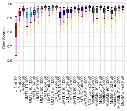
For the segmentation task, the inclusion of the saliency bridge module yields large improvements over the baseline U-Net and UMTL models. Again, with , we observed a 30% performance gain over its counterparts, which proves the effectiveness of our MultiMix model. The improvement in Dice scores of MultiMix with minimal supervision over the segmentation baselines of U-Net, UMTL, and UMTL-S is statistically significant (), confirming the quantitative efficacy of MultiMix. Figure 3 shows improved and consistent segmentation performance by the MultiMix model over the baselines. For a fair comparison, we used the same backbone U-Net and the same classification branch for all the models.
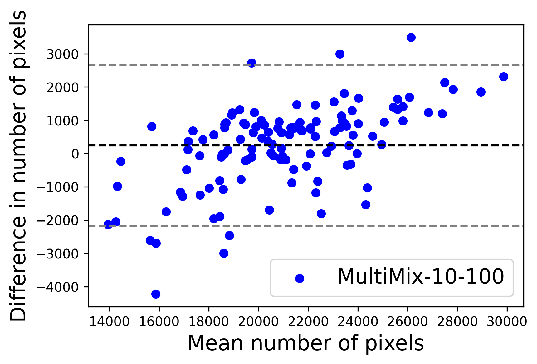
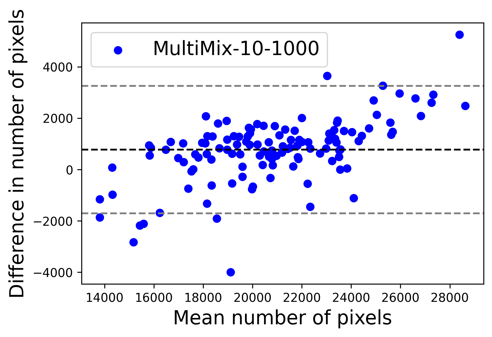
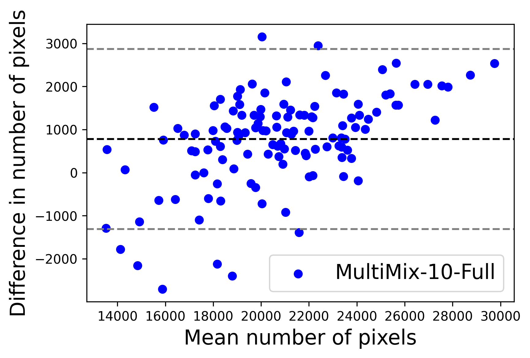
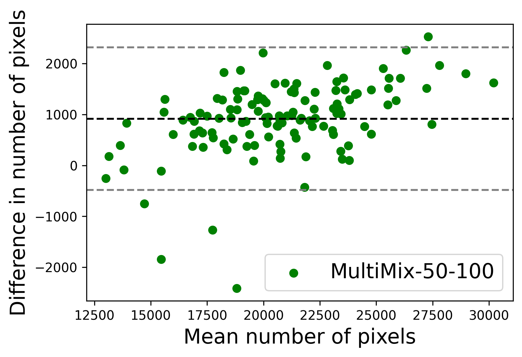
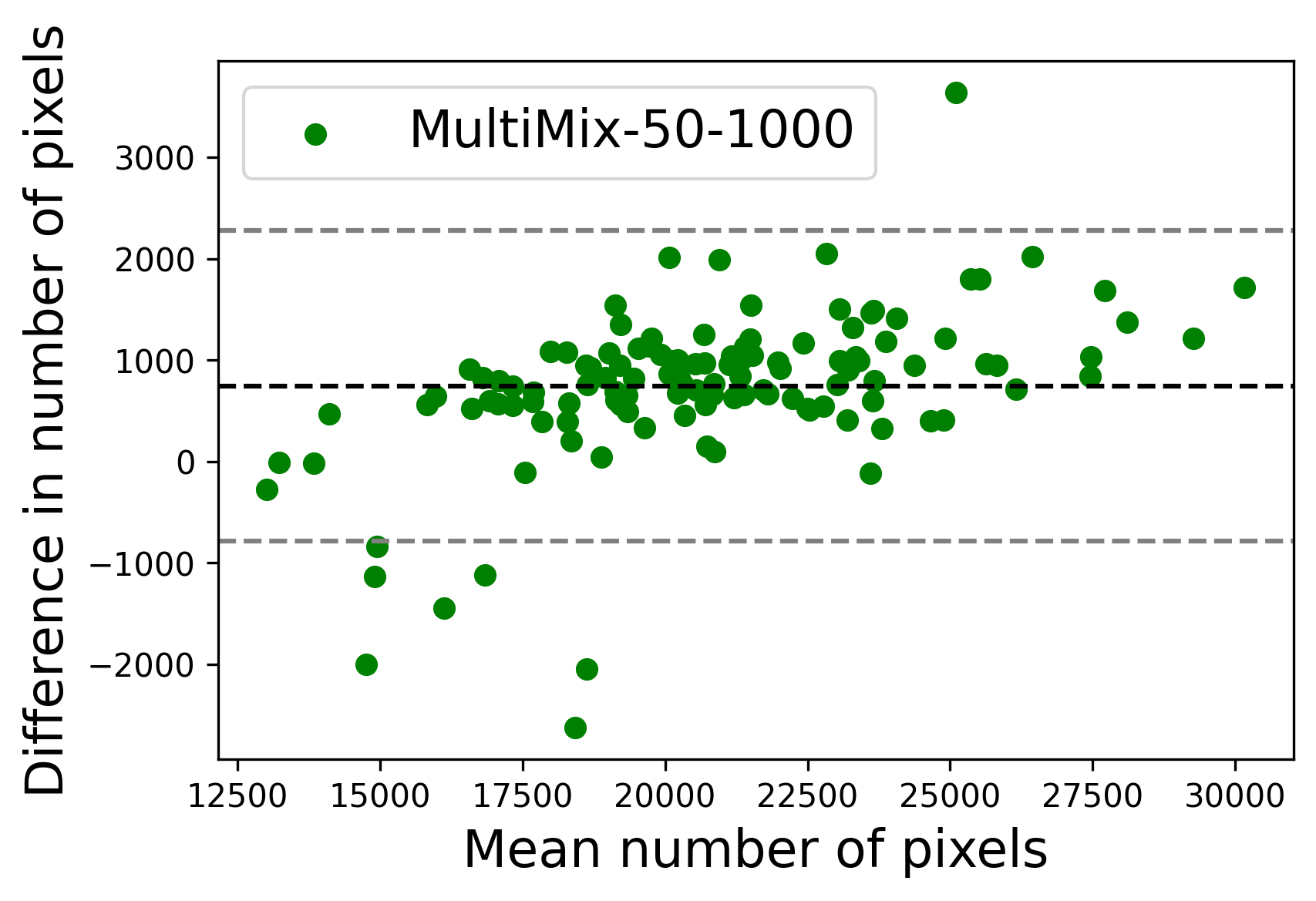
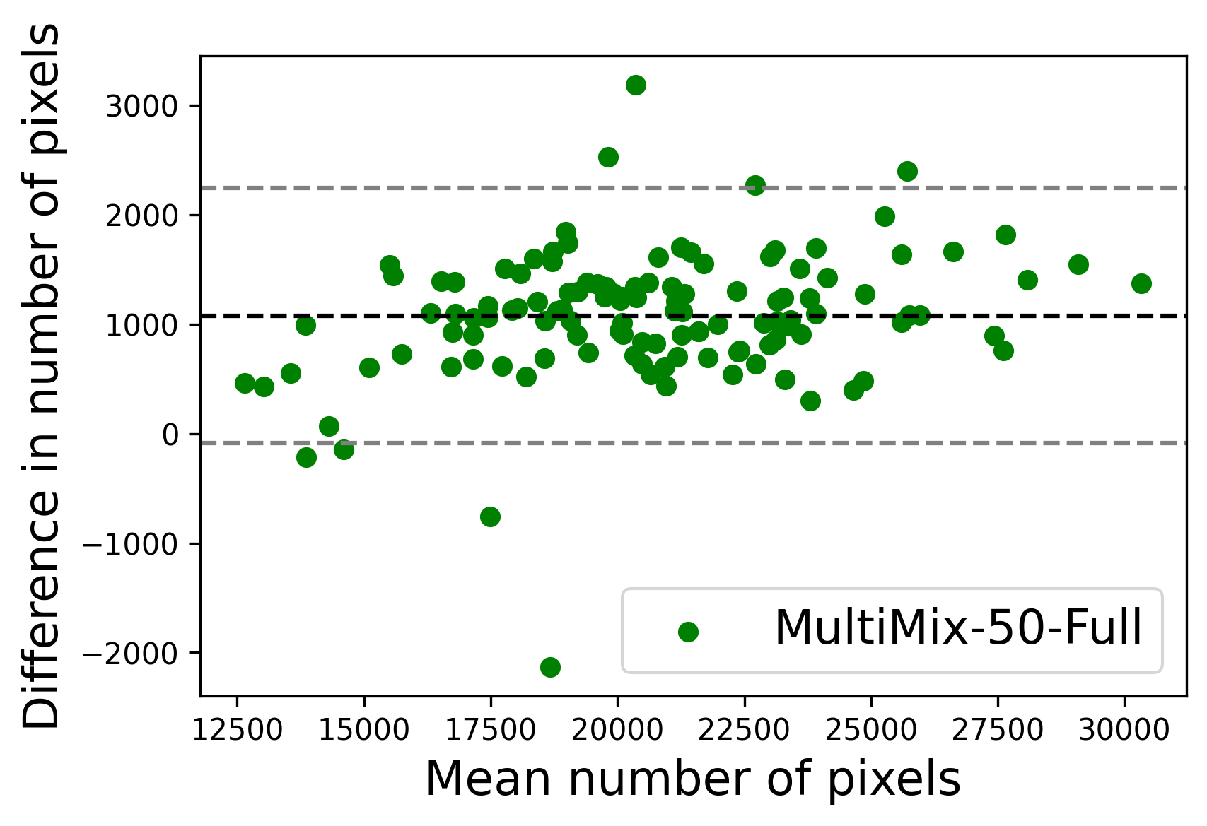
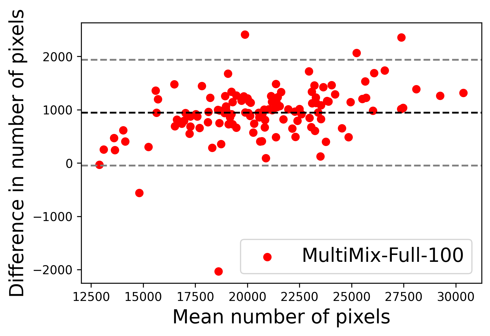
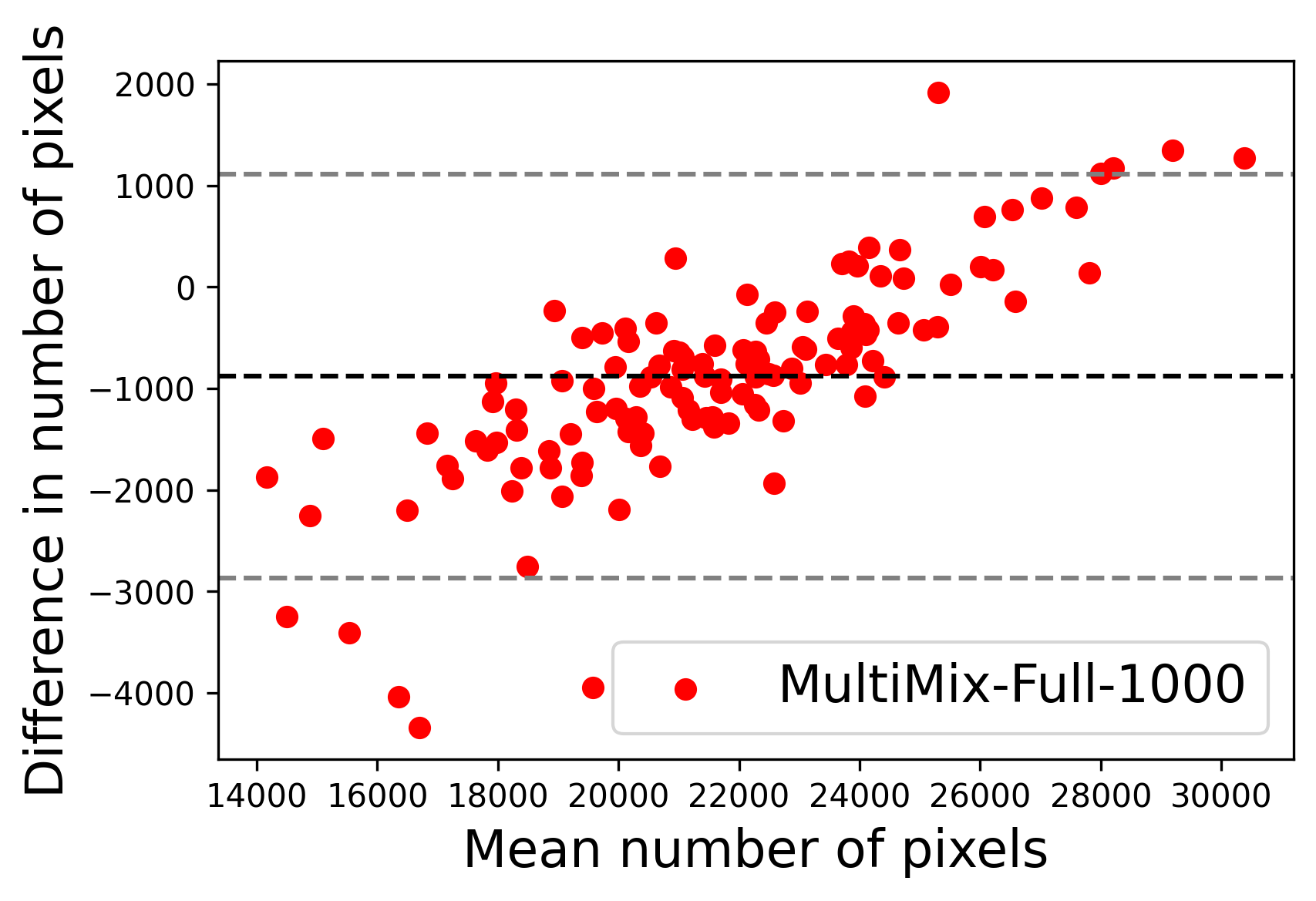
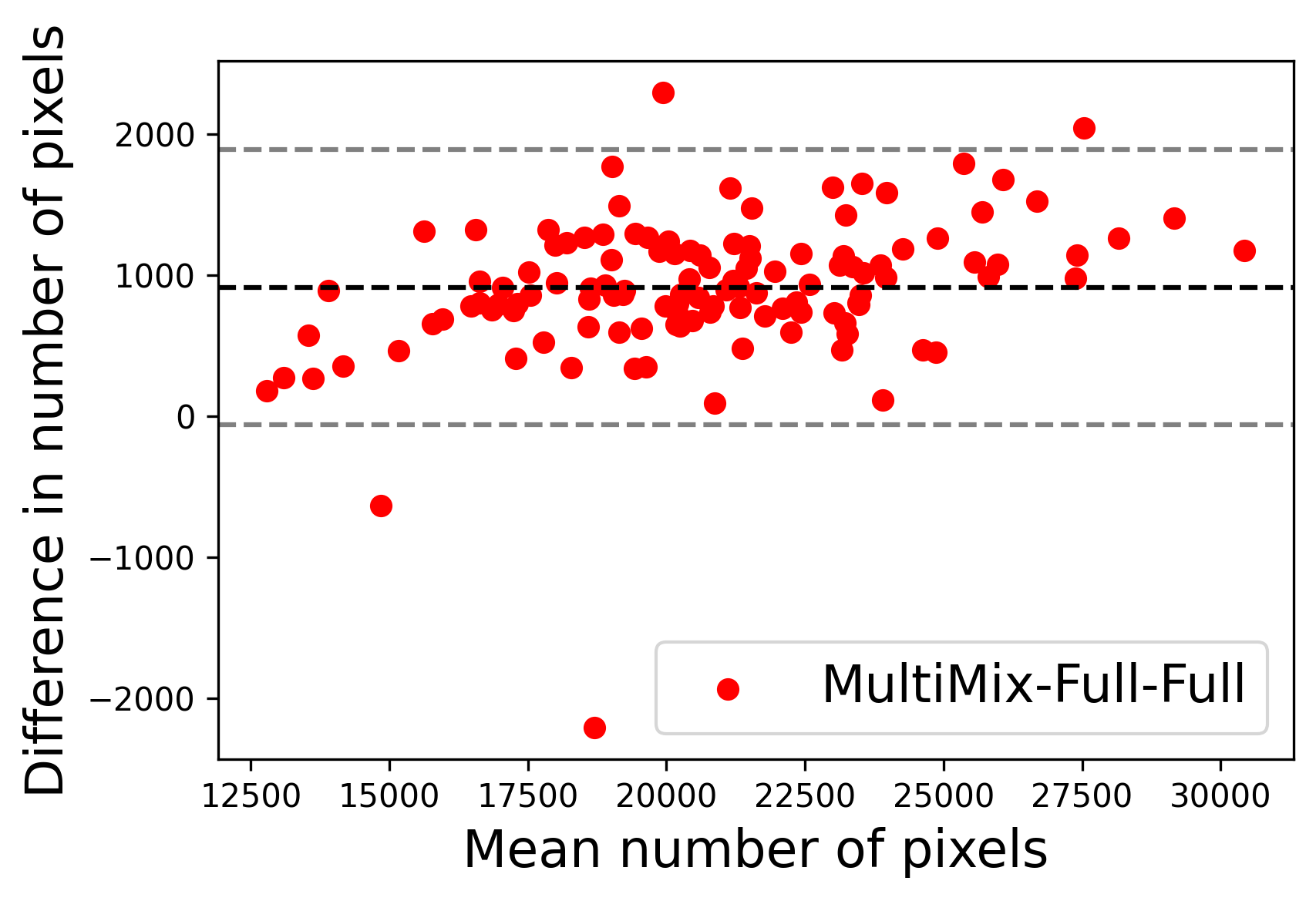
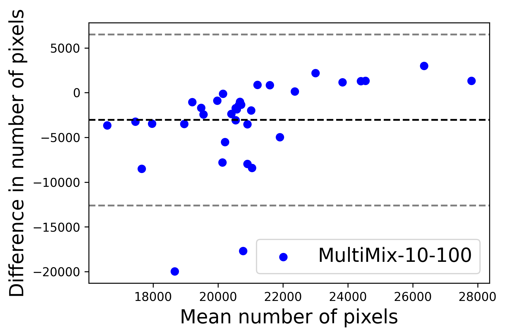
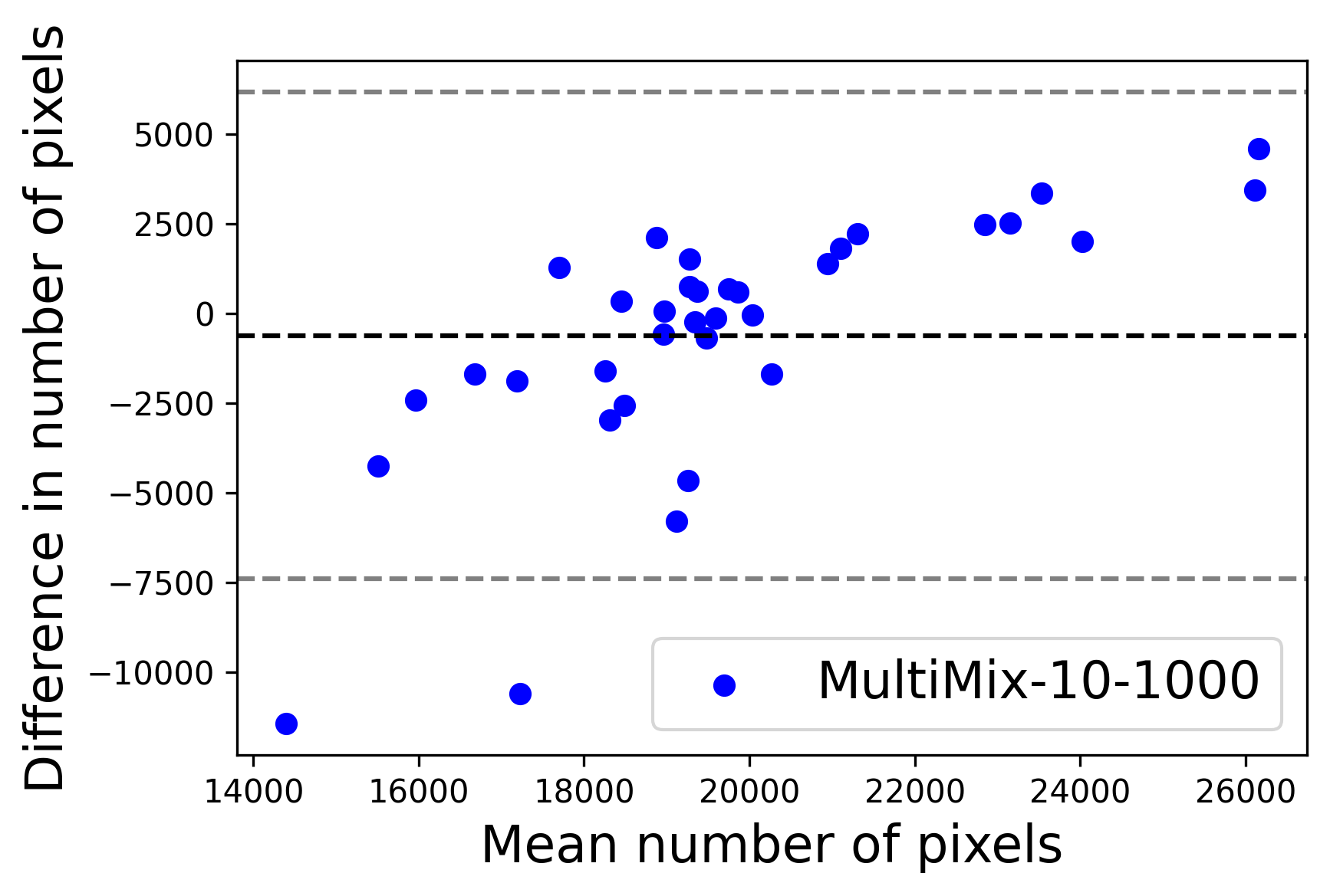
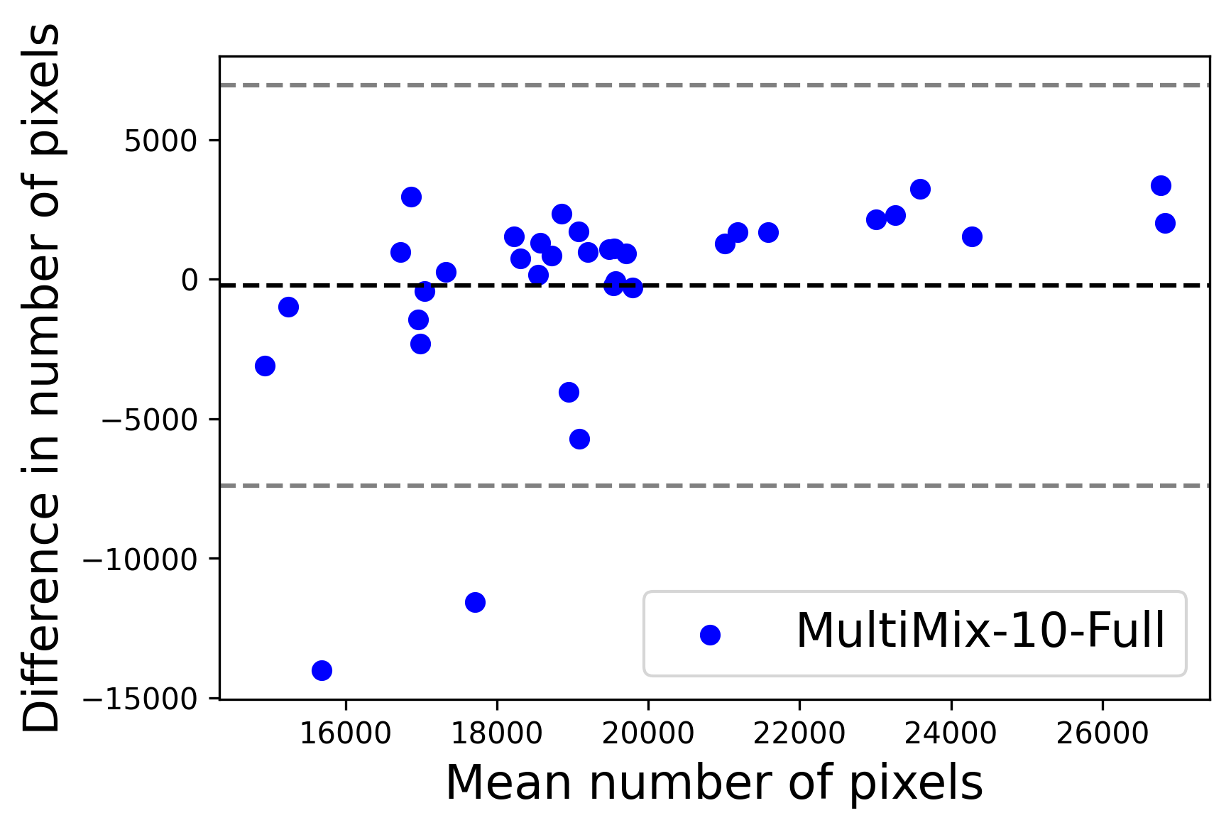
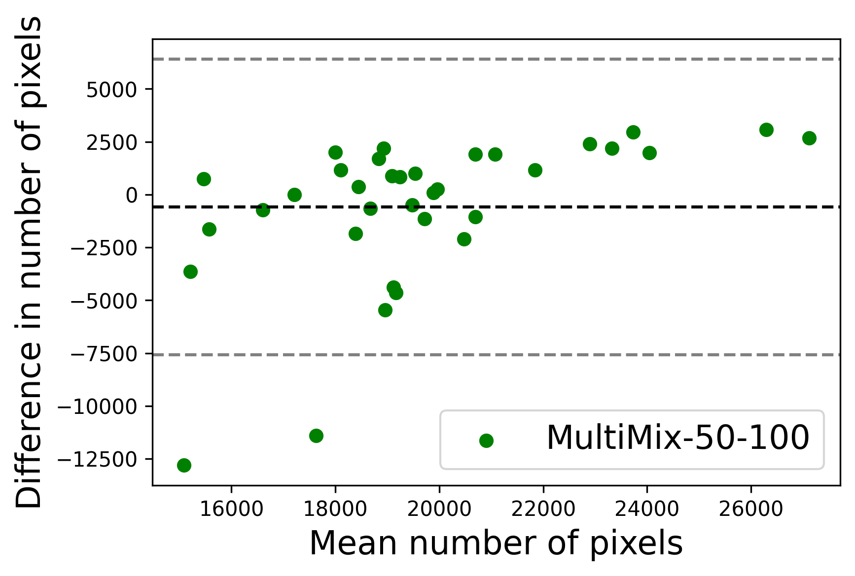
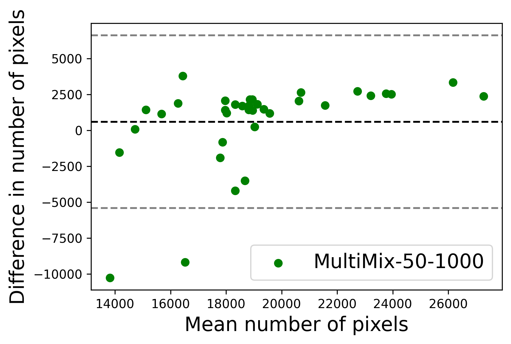
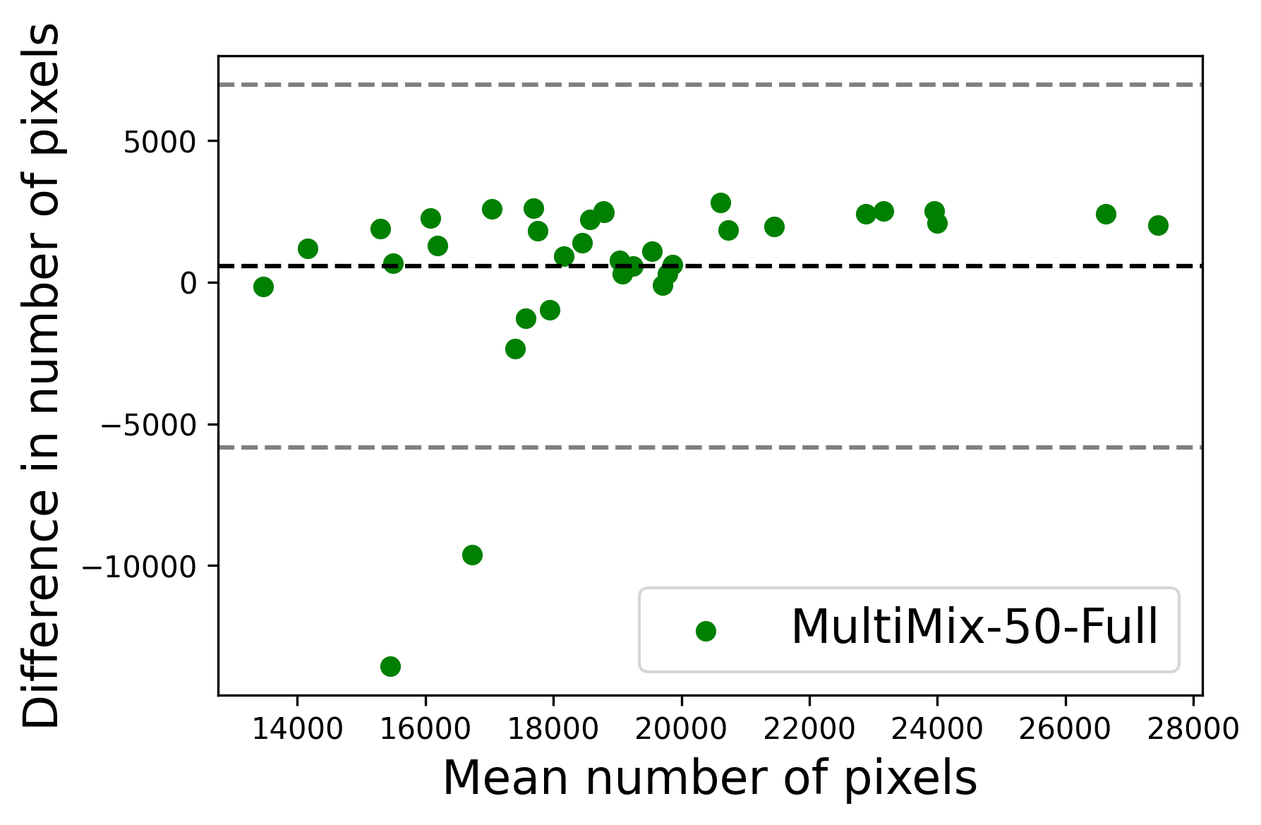
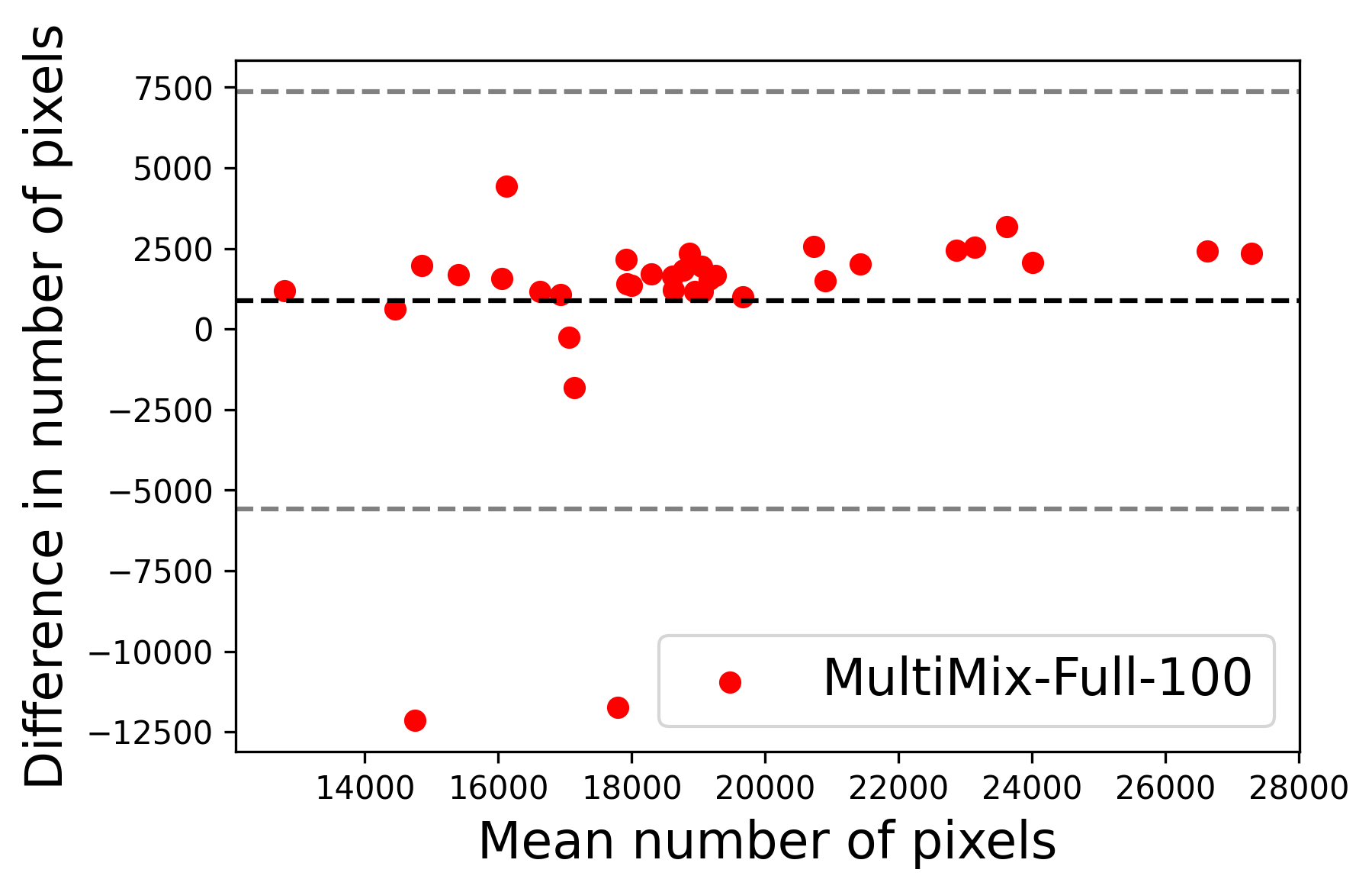
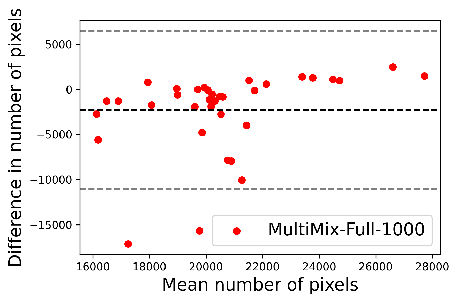
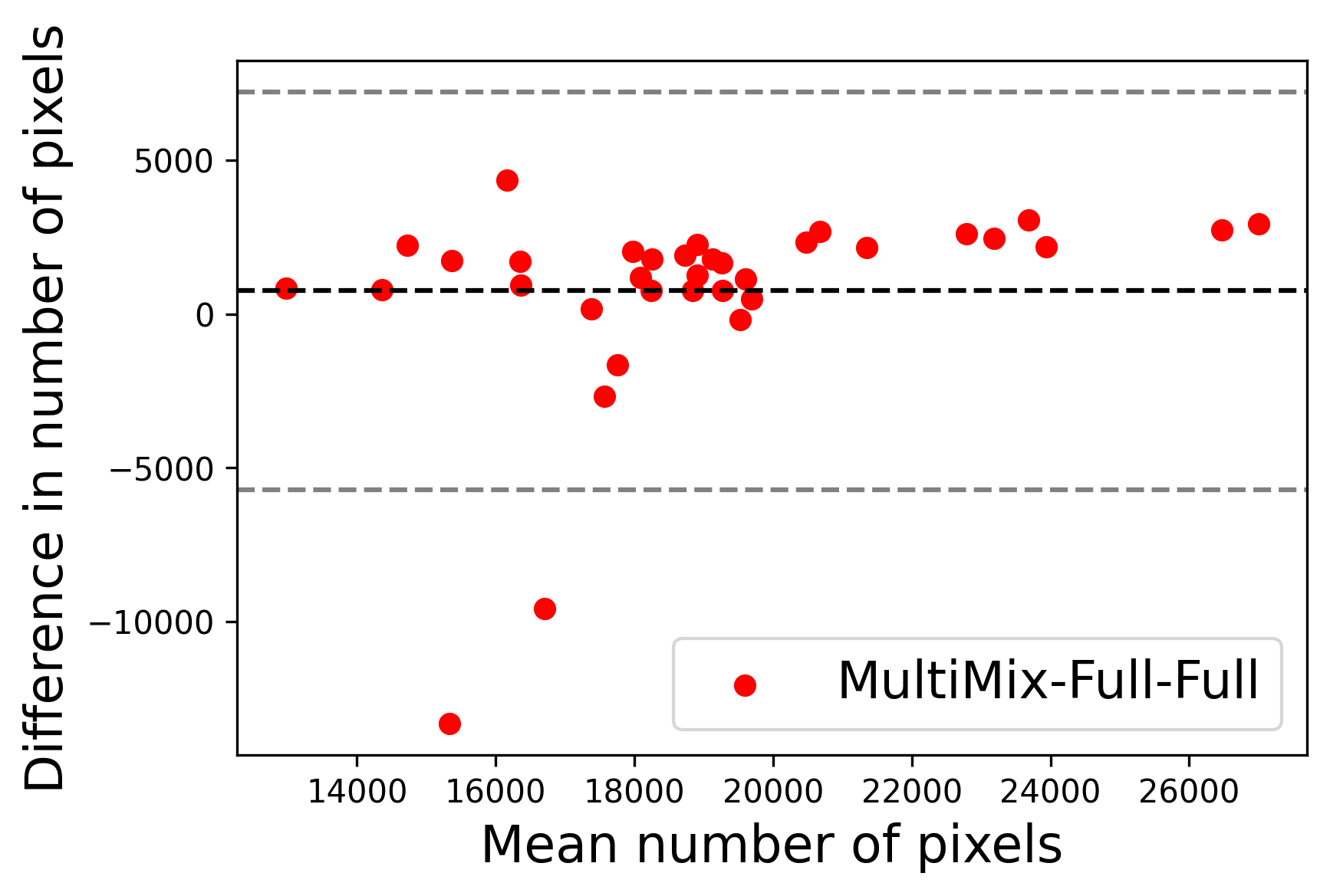
In Figure 4, the segmented lung boundary visualizations also show good agreement with the reference masks by MultiMix over the other models (also see Appendix B). For both the in-domain and cross-domain segmentations, we observe that the predicted boundaries are almost identical with the reference boundaries, as they substantially overlap. Moreover, the noise in the predictions is mitigated with the introduction of each additional component into the intermediate models, which justifies the value of those components in the MultiMix model. The good agreement between the ground truth lung masks and the MultiMix predicted segmentation masks is confirmed by the Bland-Altman plots for varying quantities of labeled data, shown in Figure 5(a).
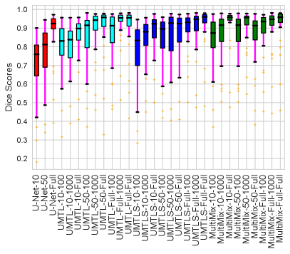
The generalization test through the cross-domain datasets (MCU and NIHX) demonstrates the effectiveness of the MultiMix model. It consistently performs well against both domains with improved generalizability in either task. As reported in Table 3, the performance of MultiMix is as promising as in the in-domain evaluations. MultiMix achieved better scores in the classification task over all the baseline models. Due to the significant differences in the NIHX and CheX datasets, the scores are not as good as the in-domain results, yet our model performs significantly better than the other classification models Enc, Enc-SSL, and UMTL (). For the segmentation task, our MultiMix model again achieved better scores in all the various metrics, with improved consistency over the baselines (Figure 3). Just like for the in-domain results, MultiMix shows significant improvements in Dice scores over the segmentation baselines U-Net, UMTL, and UMTL-S (), thus proving the generalizability of our method. The Bland-Altman plots in Figure 5(b) for the MultiMix model in the cross-domain segmentation evaluations with varying quantities of labeled data confirms the observed good agreement between the ground truth lung segmentation masks and the MultiMix-predicted segmentation masks.
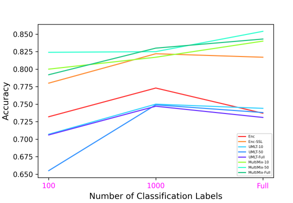
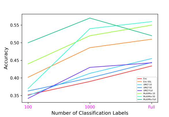
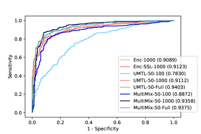
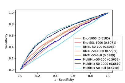
Figure 6 demonstrates the superiority and better consistency of our MultiMix models over the baselines in classifying normal and abnormal (pneumonia) X-rays. Figure 7 further showcases the superior classification performance of MultiMix over the baseline single-task and multi-task models. Figure 6 and Figure 7 together show that MultiMix outperforms all baselines in many different metrics, as the Accuracy and Area Under Curve (AUC) values confirm the superiority of the MultiMix model. With regard to the cross-domain ROC curves, however, although MultiMix has the best relative performance when compared to the baselines, the absolute performance of the algorithm indicates room for improvement.
4 Conclusions
We have presented MultiMix, a novel semi-supervised, multi-task learning model that jointly learns classification and segmentation tasks. Through the incorporation of confidence-guided data augmentation and a novel saliency bridge module, MultiMix performs improved and consistent pneumonia detection and lung segmentation when trained on multi-source chest X-ray datasets with varying quantities of ground truth labels. Our thorough experimentation using four different chest X-ray datasets demonstrated the effectiveness of MultiMix both in in-domain and cross-domain evaluations, for both tasks; in fact, outperforming a number of baseline models.
Beyond chest X-rays—which is the most frequently performed radiologic procedure worldwide, comprising 40% of all imaging tests, or 1.4 billion annually (World Health Organization, 2016)—our future work will focus on generalizing the MultiMix concept, particularly the saliency bridge module, to other applications and imaging modalities, including volumetric images.
Ethical Standards
Appropriate ethical standards were maintained in writing this manuscript and conducting the reported research, following all applicable laws and regulations regarding the treatment of animals or human subjects.
Conflicts of Interest
DT is a founder of VoxelCloud, Inc., Los Angeles, CA, USA.
A Model Architecture
Architectural details of the MultiMix model are presented in Table 4 for the encoder network and in Table 5 for the decoder network. The encoder and decoder incorporate double-convolution blocks; the encoder has 5 blocks and the decoder has 4. Each block includes a 2D convolutional layer, an instance normalization layer, and a Leaky ReLU activation, and this sequence repeats in each block.
In the encoder, each double-convolution block is followed by a dropout layer and a maxpooling layer. The encoder finally branches to a classification branch, which includes a maxpooling layer (5), an average pooling layer, followed by a fully-connected layer for classification prediction.
The decoder begins with an upsampling layer. Next, in the first double-convolution layer, the downsampled saliency maps and original inputs are concatenated. The increase in dimensions at the beginning of each decoder block are due to the skip connections. These convolutional layers are also followed by a dropout layer. This sequence is repeated for 3 more layers. To output the final segmentation prediction, the decoder finishes with a single convolutional layer that downsamples to a single channel.
B Segmentation Visualization
Figure 8 shows the ground truth lung masks and masks predicted by the MultiMix model (MultiMix-50-1000) for a number of images from the JSRT dataset (in-domain) and MCU dataset (cross-domain). Both parts of the figure display the accuracy in the predicted segmentation masks, both in-domain and cross-domain, as there is almost no noise in these predictions, proving the effectiveness of our algorithm even when being trained with limited labeled data.
C Saliency Visualization
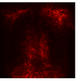
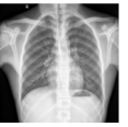
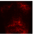
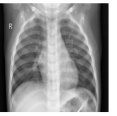
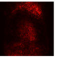
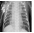
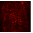
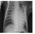
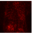
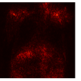
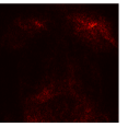
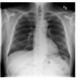
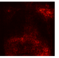
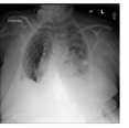
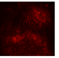
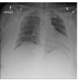
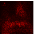
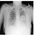
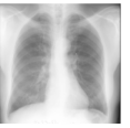
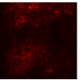
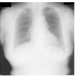
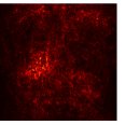
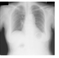
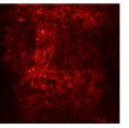
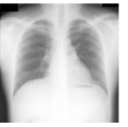
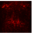
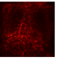
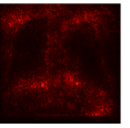
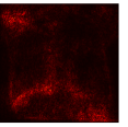
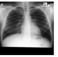
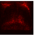
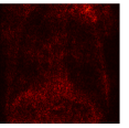
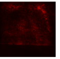
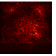
Figure 9 shows the class-specific saliency maps generated by our MultiMix-50-1000 model for both in-domain and cross-domain classification data (). The maps consistently highlight particular regions in the input X-rays for the Normal and Pneumonia classes. Similarly, Figure 10 shows the saliency maps for the in-domain and cross-domain segmentation data (). While the class labels are not available, two distinct types of saliency maps are generated like for the classification data.
Class-specific saliency maps generated for images in consistently highlight regions responsible for predicting the particular classes of the images (Figure 9), enabling the use of these maps to improve the segmentation of images in (Figure 10).
| Name | Input Feature Maps | Output Feature Maps |
|---|---|---|
| Conv layer - 1 | ||
| InstanceNorm - 1 | ||
| LReLU - 1 | ||
| Conv Layer - 2 | ||
| InstanceNorm - 2 | ||
| LReLU - 2 | ||
| Dropout - 1 | ||
| Maxpool - 1 | ||
| Conv Layer - 3 | ||
| InstanceNorm - 3 | ||
| LReLU - 3 | ||
| Conv Layer - 4 | ||
| InstanceNorm - 4 | ||
| LReLU - 4 | ||
| Dropout - 2 | ||
| Maxpool - 2 | ||
| Conv Layer - 5 | ||
| InstanceNorm - 5 | ||
| LReLU - 5 | ||
| Conv Layer - 6 | ||
| InstanceNorm - 6 | ||
| LReLU - 6 | ||
| Dropout - 3 | ||
| Maxpool - 3 | ||
| Conv Layer - 7 | ||
| InstanceNorm - 7 | ||
| LReLU - 7 | ||
| Conv Layer - 8 | ||
| InstanceNorm - 8 | ||
| LReLU - 8 | ||
| Dropout - 4 | ||
| Maxpool - 4 | ||
| Conv Layer - 9 | ||
| InstanceNorm - 9 | ||
| LReLU - 9 | ||
| Conv Layer - 10 | ||
| InstanceNorm - 10 | ||
| LReLU - 10 | ||
| Dropout - 5 | ||
| Maxpool - 5 | ||
| Avgpool | ||
| GAP | ||
| Fully Connected Layer |
| Name | Input Feature Maps | Output Feature Maps |
|---|---|---|
| Upsample - 1 | ||
| Conv Layer - 1 | ||
| InstanceNorm - 1 | ||
| LReLU - 1 | ||
| Conv Layer - 2 | ||
| InstanceNorm - 2 | ||
| LReLU - 2 | ||
| Dropout - 1 | ||
| Upsample - 2 | ||
| Conv Layer - 3 | ||
| InstanceNorm - 3 | ||
| LReLU - 3 | ||
| Conv Layer - 4 | ||
| InstanceNorm - 4 | ||
| LReLU - 4 | ||
| Dropout - 2 | ||
| Upsample - 3 | ||
| Conv Layer - 5 | ||
| InstanceNorm - 5 | ||
| LReLU - 5 | ||
| Conv Layer - 6 | ||
| InstanceNorm - 6 | ||
| LReLU - 6 | ||
| Dropout - 3 | ||
| Upsample - 4 | ||
| Conv Layer - 7 | ||
| InstanceNorm - 7 | ||
| LReLU - 7 | ||
| Conv Layer - 8 | ||
| InstanceNorm - 8 | ||
| LReLU - 8 | ||
| Dropout - 4 | ||
| Final Conv Layer |
| Image | Ground Truth | Prediction |
|---|---|---|
| Image | Ground Truth | Prediction |
|---|---|---|
| Image | Saliency Map |
| Normal | |
 |  |
 |  |
 |  |
| Pneumonia | |
 |  |
 |  |
 |  |
| Image | Saliency Map |
| Normal | |
 |  |
 |  |
 |  |
| Pneumonia | |
 |  |
 |  |
 |  |
| Image | Saliency Map |
|---|---|
 |  |
 |  |
 |  |
 |  |
 |  |
 |  |
| Image | Saliency Map |
|---|---|
 |  |
 |  |
 |  |
 |  |
 |  |
 |  |
References
- Anwar et al. (2018) S. M. Anwar, M. Majid, A. Qayyum, M. Awais, M. Alnowami, and M. K. Khan. Medical image analysis using convolutional neural networks: A review. Journal of Medical Systems, 42(11):226, 2018.
- Beijbom (2012) O. Beijbom. Domain adaptations for computer vision applications. arXiv Preprint arXiv:1211.4860, 2012.
- Berthelot et al. (2019) D. Berthelot, N. Carlini, I. Goodfellow, N. Papernot, A. Oliver, and C. Raffel. Mixmatch: A holistic approach to semi-supervised learning. arXiv Preprint arXiv:1905.02249, 2019.
- Caruana (1993) R. A. Caruana. Multitask learning: A knowledge-based source of inductive bias. In Proceedings of the International Conference on Machine Learning, pages 41–48, 1993.
- Chapelle et al. (2009) O. Chapelle, B. Scholkopf, and A. Zien. Semi-supervised learning (chapelle, o. et al., eds.; 2006)[book reviews]. IEEE Transactions on Neural Networks, 20(3):542–542, 2009.
- Gao et al. (2019) F. Gao, H. Yoon, T. Wu, and X. Chu. A feature transfer enabled multi-task deep learning model on medical imaging. arXiv Preprint arXiv:1906.01828, 2019.
- Girard et al. (2019) F. Girard, C. Kavalec, and F. Cheriet. Joint segmentation and classification of retinal arteries/veins from fundus images. Artificial Intelligence in Medicine, 94:96–109, Mar 2019.
- Grandvalet and Bengio (2005) Y. Grandvalet and Y. Bengio. Semi-supervised learning by entropy minimization. In Advances in Neural Information Processing Systems, pages 529–536, 2005.
- Gu et al. (2019) Z. Gu, J. Cheng, H. Fu, K. Zhou, H. Hao, Y. Zhao, T. Zhang, S. Gao, and J. Liu. CE-Net: Context encoder network for 2D medical image segmentation. IEEE Transactions on Medical Imaging, 38(10):2281–2292, 2019.
- Haque et al. (2021) A. Haque, A.-A.-Z. Imran, A. Wang, and D. Terzopoulos. Multimix: Sparingly supervised, extreme multitask learning from medical images. In Proceedings of the IEEE International Symposium on Biomedical Imaging (ISBI), pages 693–696, Nice, France, April 2021.
- Hu et al. (2019) J. Hu, H. Wang, S. Gao, M. Bao, T. Liu, Y. Wang, and J. Zhang. S-unet: A bridge-style U-Net framework with a saliency mechanism for retinal vessel segmentation. IEEE Access, 7:174167–174177, 2019. doi: 10.1109/ACCESS.2019.2940476.
- Imran (2020) A.-A.-Z. Imran. From Fully-Supervised, Single-Task to Scarcely-Supervised, Multi-Task Deep Learning for Medical Image Analysis. PhD thesis, Computer Science Department, University of California, Los Angeles, 2020.
- Imran and Terzopoulos (2019) A.-A.-Z. Imran and D. Terzopoulos. Semi-supervised multi-task learning with chest X-ray images. In Proceedings of the 10th International Workshop on Machine Learning in Medical Imaging (MLMI 2019), volume 11861 of Lecture Notes in Computer Science, pages 98–105. Springer Nature, 2019.
- Imran and Terzopoulos (2021a) A.-A.-Z. Imran and D. Terzopoulos. Progressive adversarial semantic segmentation. In Proceedings of the 25th International Conference on Pattern Recognition (ICPR), pages 4910–4917, Milan, Italy, January 2021a.
- Imran and Terzopoulos (2021b) A.-A.-Z. Imran and D. Terzopoulos. Multi-adversarial variational autoencoder nets for simultaneous image generation and classification. In Deep Learning Applications, Volume 2, pages 249–271. Springer, 2021b.
- Imran et al. (2020) A.-A.-Z. Imran, C. Huang, H. Tang, W. Fan, Y. Xiao, D. Hao, Z. Qian, and D. Terzopoulos. Partly supervised multi-task learning. In Proceedings of the 19th IEEE International Conference on Machine Learning and Applications (ICMLA), pages 769–774, Miami, FL, December 2020.
- Jaeger et al. (2014) S. Jaeger, S. Candemir, et al. Two public chest X-ray datasets for computer-aided screening of pulmonary diseases. Quantitative Imaging in Medicine and Surgery, 2014.
- Kermany et al. (2018) D. S. Kermany, M. Goldbaum, W. Cai, C. C. S. Valentim, H. Liang, S. L. Baxter, A. McKeown, G. Yang, X. Wu, F. Yan, et al. Identifying medical diagnoses and treatable diseases by image-based deep learning. Cell, 172(5):1122–1131, 2018.
- Lee (2013) D.-H. Lee. Pseudo-label: The simple and efficient semi-supervised learning method for deep neural networks. In ICML Workshop on Challenges in Representation Learning, volume 3, pages 1–6, 2013.
- Liu et al. (2008) Q. Liu, X. Liao, and L. Carin. Semi-supervised multitask learning. In Advances in Neural Information Processing Systems, pages 937–944, 2008.
- Mehta et al. (2018) S. Mehta, E. Mercan, J. Bartlett, D. Weave, J. G. Elmore, and Shapiro L. Y-Net: Joint segmentation and classification for diagnosis of breast biopsy images. arXiv Preprint arXiv:1806.01313, 2018.
- Myronenko (2018) A. Myronenko. 3D MRI brain tumor segmentation using autoencoder regularization. arXiv Preprint arXiv:1810.11654, 2018.
- Ouali et al. (2020) Y. Ouali, C. Hudelot, and M. Tami. An overview of deep semi-supervised learning. arXiv Preprint arXiv:2006.05278, 2020.
- Ronneberger et al. (2015) O. Ronneberger, P. Fischer, and T. Brox. U-Net: Convolutional networks for biomedical image segmentation. arXiv Preprint arXiv:1505.04597, 2015.
- Ruder (2017) S. Ruder. An overview of multi-task learning in deep neural networks. arXiv Preprint arXiv:1706.05098, 2017.
- Salimans et al. (2016) T. Salimans, I. Goodfellow, W. Zaremba, V. Cheung, A. Radford, and X. Chen. Improved techniques for training GANs. arXiv Preprint arXiv:1606.03498, 2016.
- Shiraishi et al. (2000) J. Shiraishi, S. Katsuragawa, et al. Development of a digital image database for chest radiographs with and without a lung nodule. American Journal of Roentgenology, 174:71–74, 2000.
- Simonyan et al. (2014) K. Simonyan, A. Vedaldi, and A. Zisserman. Deep inside convolutional networks: Visualising image classification models and saliency maps. arXiv Preprint arXiv:1312.6034, 2014.
- Sohn et al. (2020) K. Sohn, D. Berthelot, C.-L. Li, Z. Zhang, N. Carlini, E. D. Cubuk, A. Kurakin, H. Zhang, and C. Raffel. FixMatch: Simplifying semi-supervised learning with consistency and confidence. arXiv Preprint arXiv:2001.07685, 2020.
- Wang et al. (2017) X. Wang, Y. Peng, L. Lu, Z. Lu, M. Bagheri, and R. M. Summers. ChestX-Ray8: Hospital-scale chest X-ray database and benchmarks on weakly-supervised classification and localization of common thorax diseases. In Proceedings of the IEEE Conference on Computer Vision and Pattern Recognition (CVPR), pages 2097–2106, 2017.
- World Health Organization (2016) World Health Organization. Communicating radiation risks in paediatric imaging, 2016. URL https://www.who.int/publications/i/item/978924151034.
- Zeng et al. (2019) Y. Zeng, Y. Zhuge, H. Lu, and L. Zhang. Joint learning of saliency detection and weakly supervised semantic segmentation. In Proceedings of the IEEE/CVF International Conference on Computer Vision, pages 7223–7233, 2019.
- Zhang et al. (2016) D. Zhang, D. Meng, L. Zhao, and J. Han. Bridging saliency detection to weakly supervised object detection based on self-paced curriculum learning. In Proceedings of the International Joint Conference on Artificial Intelligence (IJCAI), 2016.
- Zhou et al. (2019) Y. Zhou, X. He, L. Huang, L. Liu, F. Zhu, S. Cui, and L. Shao. Collaborative learning of semi-supervised segmentation and classification for medical images. In Proceedings of the IEEE Conference on Computer Vision and Pattern Recognition (CVPR), June 2019.