
1 Introduction
A contemporary key element in building automated pathology detection systems with machine learning in medical imaging is the availability and accessibility of a sufficient amount of data in order to train supervised discriminator models for accurate results. This is a problem in medical imaging applications, where data accessibility is scarce because of regulatory constraints and economic considerations. To build truly useful diagnostic systems, supervised machine learning methods would require a large amount of data and manual labelling effort for every possible disease to minimise false predictions. This is unrealistic because there are thousands of diseases, some represented only by a few patients ever recorded. Thus, learning representations from healthy anatomy and using anomaly detection to flag unusual image features for further investigation defines a more reasonable paradigm for medicine, especially in high-throughput settings like population screening, e.g. fetal ultrasound imaging. However, anomaly detection suffers from the great variability of healthy anatomical structures from one individual to another within patient populations as well as from the many, often subtle, variants and variations of pathologies. Many medical imaging datasets, e.g. volunteer studies like UK Biobank (Petersen et al., 2013), consist of images from predominantly healthy subjects with a small proportion of them belonging to abnormal cases. Thus, an anomaly detection approach or ’normative’ learning paradigm is also reasonable from a practical point of view for applications like quality control within massive data lakes.
In this work, we formulate the detection of congenital heart disease as an anomaly detection task for fetal screening with ultrasound imaging. We utilise normal control data to learn the normative feature distribution which characterises healthy hearts and distinguishes them from fetuses with hypoplastic left heart syndrome (HLHS). We chose this test pathology because of our access to a well labelled image database from this domain. Theoretically, our method could be evaluated on any congenital heart disease that is visible in the four-chamber view of the heart (NHS, 2015).
Contribution: To the best of our knowledge we propose the first unsupervised working anomaly detection approach for fetal ultrasound screening using only normal samples during training. Previous approaches rely on supervised (Arnaout et al., 2020) discrimination of known diseases, which makes them prone to errors when confronted with unseen classes. Our method extends the -GAN architecture with attention mechanisms and we propose an anomaly score which is based on reconstruction and localisation capabilities of the model. We evaluate our method on a selected congenital heart disease, which can be overlooked during clinical screening examinations in between 30-40% of scans (Chew et al., 2007), and compare to other state-of-the-art methods in image-based anomaly detection. We show evidence that the proposed method outperforms state-of-the-art models and achieves promising results for unsupervised detection of pathologies in fetal ultrasound screening.
2 Background and Related Work
2.1 Pathological Diseases in Fetal Heart
Congenital heart disease (CHD) is the most common group of congenital malformations (Bennasar et al., 2010)(Yeo et al., 2018)(van Velzen et al., 2016). CHD is a defect in the structure of the heart or great vessels that is present at birth. Approximately per newborns are affected. of these heart defects require surgery within the first year of life (Yeo et al., 2018). In order to detect the disease, the most common approach is the standard anomaly ultrasound scan at approximately weeks of gestation (e.g. 18+0 to 20+6 weeks in the UK). In contemporary screening pathways, i.e., 2D ultrasound at GA 12 and 24, the prenatal detection rate of CHD is in a range of . (Pinto et al., 2012) (van Velzen et al., 2016) In (Yeo et al., 2018), algorithmic support has been used to find diagnostically informative fetal cardiac views. With this aid, clinical experts have been shown to discriminate healthy controls from CHD cases with sensitivity and specificity in 4D ultrasound. However, 4D ultrasound is not commonly used during fetal screening and in the proposed teleradiology setup still all images have to be manually assessed by highly experienced experts to achieve such a high performance.
In this work we focus on a subtype of CHD, Hypoplastic Left Heart Syndrome (HLHS). Examples of HLHS in comparison with healthy fetal hearts are presented in Figure 1. HLHS is rare, but is one of the most prominent pathologies in our cohort. In HLHS the four chamber view is usually grossly abnormal, allowing the identification of CHD (although not necessarily a detailed diagnosis) from a single image plane. A condition that is identifiable on a single view plane provides a clear case study for our proposed method. If HLHS is identified during pregnancy, provisions for the appropriate timing and location of delivery can be made, allowing immediate treatment of the affected infant to be instigated after birth. Postnatal palliative surgery is possible for HLHS, and the antenatal diagnosis of CHD in general has been shown to result in a reduced mortality compared to those infants diagnosed with CHD only after birth (Holland et al., ). However, the detection of this pathology during routine screening still remains challenging. Screening scans are performed by front-line-of-care sonographers with varying degrees of experience and the examination is influenced by factors such as fetal motion and the small size of the fetal heart.

2.2 One-class anomaly detection methods in Medical Imaging
One-class classification is a case of multi-class classification where the data is from a single class. The main goal is to learn either a representation or a classifier (or a combination of both) in order to distinguish and recognise out-of-distribution samples during inference. Discriminative as well as generative methods have been proposed utilizing deep learning, for example one class CNN (Oza and Patel, 2019) and Deep SVDD (Ruff et al., 2018). Usually these methods utilise loss functions, similar to those of OC-SVM (Schölkopf et al., 2001) and SVDD (Tax and Duin, 2004) or use regularisation techniques to make conventional neural networks compatible to one-class classification models (Perera et al., 2021). Generative models are mostly based on autoencoders or Generative Adversarial Networks. In this work we mainly focus on the application of generative adversarial networks for anomaly detection in medical imaging.
Generative adversarial networks for anomaly detection were first proposed by (Schlegl et al., 2017). In (Schlegl et al., 2017), a deep convolutional generative adversarial network, inspired by DCGAN as proposed by (Radford et al., 2016), is used as AnoGAN. During the training phase, only healthy samples are used. This approach consists of two models. A generator, which generates an image from random noise and a discriminator, which classifies real or fake samples as common in GANs. More specifically, the generator learns the mapping from the uniformly distributed input noise sampled from the latent space to the 2D image space of healthy data. The output of the discriminator is a single value, which is interpreted as the probability of an image to be real or generated by the generator network. In their work, a residual loss is introduced, which is defined as the norm between the real images and the generated image. This enforces the visual similarity between the initial image and the generated one. Furthermore, in order to cope with GAN instability, instead of optimizing the parameters of the generator via maximizing the discriminator’s output on generated examples, the generator is forced to generate data whose intermediate feature representation of the discriminator () is similar to those of real images. This is defined as the norm between intermediate feature representations of the discriminator given as input the real image and the generate image respectively. In AnoGAN, an anomaly score is defined as the loss function at the last iteration, i.e., the residual error plus the discrimination error. AnoGAN has been tested on a high-resolution SD-OCT dataset. For evaluation purposes, the authors report receiver operating characteristic (ROC) curves of the corresponding anomaly detection performance on image level. Based on their results, using the residual loss alone already yields good results for anomaly detection. The combination with the discriminator loss improves the overall performance slightly. During testing, an iterative search in the latent space is used in order to find the closest latent vector that reconstructs the real test image better. This is a time consuming procedure and this optimisation process can get stuck in local minima.
Similar to AnoGAN, a faster approach, f-AnoGAN has been proposed in (Schlegl et al., 2019). In this work, the authors train a GAN on normal images, however instead of the DCGAN model a Wasserstein GAN (WGAN) (Arjovsky et al., 2017)(Gulrajani et al., 2017) has been used. Initially, a WGAN is trained in order to learn a non-linear mapping from latent space to the image space domain. Generator and discriminator are optimised simultaneously. Samples that follow the data distribution are generated through the generator, given input noise sampled from the latent space. Then an encoder (convolutional autoencoder) is training to learn a map from image space to latent space. For the training of the encoder, different approaches are followed, i.e training an encoder with generated images (z-to-z approach-ziz), training an encoder with real images (an image-to-image mapping approach -izi) and training a discriminator guided izi encoder (). As anomaly score, image reconstruction residual plus the residual of the discriminator’s feature representation () is used. The method is evaluated on optical coherence tomography imaging data of the retina. Both (Schlegl et al., 2017) as well as (Schlegl et al., 2019) use image patches for training and are modular methods which are not trained in an end-to-end fashion.
Another GAN-based method applied to OCT data has been proposed by (Zhou et al., 2020), in which authors propose a Sparsity-constrained Generative Adversarial Network (Sparse-GAN), a network based on an Image-to-Image GAN (Isola et al., 2017). Sparse-GAN consists of a generator, following the same approach as in (Isola et al., 2017), and a discriminator. Features in the latent space are constrained using a Sparsity Regularizer Net. The model is optimized with a reconstruction loss combined with an adversarial loss. The anomaly score is computed in the latent space and not in image space. Furthermore, an Anomaly Activation Map (AAM) is proposed to visualise lesions.
Subsequently, AnoVAEGAN (Baur et al., 2018) has been proposed, in which the authors discuss a spatial variational autoencoder and a discriminator. It is applied to high resolution MRI images for unsupervised lesion segmentation. AnoVAEGAN uses a variational autoencoder and tries to model the normal data distribution that will lead the model to fully reconstruct the healthy data while it is expected to fail reconstructing abnormal samples. The discriminator classifies the inputs as real or reconstructed data. As anomaly score the norm of the original image and the reconstructed image is used.
Opposite to reconstruction-based anomaly detection methods as they are discussed above, in (Shen et al., 2020) adGAN, an alternative framework based on GANs, is proposed. The authors introduce two key components: fake pool generation and concentration loss. adGAN follows the structure of WGAN and consists of a generator and discriminator. The WGAN is first trained with gradient penalty using healthy images only and after a number of iterations a pool of fake images is collected from the current generator. Then a discriminator is retrained using the initial set of healthy data as well as the generated images in the fake pool with a concentration loss function. Concentration loss is a combination of the traditional WGAN loss function with a concentration term which aims to decrease the within-class distance of normal data. The output of the discriminator is considered as anomaly score. The method is applied to skin lesion detection and brain lesion detection. Two other methods that utilise discriminator outputs as anomaly score, however not tested for medical imaging, are ALOOC (Sabokrou et al., 2018) and fenceGAN (Ngo et al., 2019). In ALOOC (Sabokrou et al., 2018), the discriminator’s probabilistic output is utilised as abnormality score. In their work an encoder-decoder is used for reconstruction while the discriminator tries to differentiate the reconstructed images from the original ones. An extension of the ALOOC algorithm, is the Old is Gold (OGN) algorithm which is presented in (Zaheer et al., 2020). After training a framework similar to ALOOC, the authors finetune the network using two different types of fake images which are bad quality images and pseudo anomaly images. In this way they try to boost the ability of the discriminator to differentiate normal images from abnormal ones.
In (Ngo et al., 2019) the authors propose an encirclement loss that places the generated images at the boundary of the distribution and then use the discriminator in order to distinguish anomalous images. They propose this loss with the idea that a conventional GAN objective encourages the distribution of generated images to overlap with real images.
In (Gong et al., 2020) an approach based on the ALOOC algorithm is proposed for the detection of fetal congenital heart disease. However, during training both normal and abnormal samples are available, which is one of the key differences compared to our approach where only healthy subjects are utilised. Furthermore, additional to the encoder-decoder and discriminator networks which are used in ALOOC, they use two additional noise models of the same architecture where the input is an image plus Gaussian noise () in order to make their encoder-decoder networks more robust to distortions. In (Perera et al., 2019) a one-class generative adversarial network (OCGAN) is proposed for anomaly detection. OCGAN consists of two discriminators, a visual and a latent discriminator, a reconstruction network (denoising autoencoder) and a classifier. The latent discriminator learns to discriminate encoded real images and generated images randomly sampled from , while the visual discriminator distinguishes real from fake images. Their classifier is trained using binary cross entropy loss and learns to recognise real images from fake images. Finally, in (Pidhorskyi et al., 2018) a probabilistic framework is proposed which is based on a model similar to -GAN. The latent space is forced to be similar to standard normal distribution through an extra discriminator network, called latent discriminator similar to (Rosca et al., 2017). A parameterized data manifold is defined (using adversarial autoencoder) which captures the underlying structure of the inlier distribution (normal data) and a test sample is considered as abnormal if its probability with respect to the inlier distribution is below a threshold. The probability is factorised with respect to local coordinates of the manifold tangent space.
A summary of the key features for the works above is given in Table 1.
To establish consistency between different related works we define as a test image, as a reconstructed image, as a discriminator network, ( as (intermediate) feature representation of a Discriminator network), as an encoder network (image space latent space), as a decoder network (latent space back to image space), as a generator network (where input is a noise vector), as latent space representation and as a fixed learning rate.
| Reference | Approach | Anomaly score | Dataset |
|---|---|---|---|
| AnoGAN (Schlegl et al., 2017) | reconstruction & discrimination score | OCT | |
| f-AnoGAN (Schlegl et al., 2019) | reconstruction & discrimination score | OCT | |
| Sparse-GAN (Zhou et al., 2020) | reconstruction error | OCT | |
| AnoVAEGAN (Baur et al., 2018) | reconstruction error | Brain | |
| adGAN (Shen et al., 2020) | discriminator score | Digit/skin/Brain | |
| ALOOC (Sabokrou et al., 2018) | discriminator score | Generic Images/Video | |
| fenceGAN (Ngo et al., 2019) | discriminator score | Generic Images | |
| OGN (Zaheer et al., 2020) | discriminator score | Generic Images/Video | |
| OCGAN (Perera et al., 2019) | discriminator/reconstruction score | / | Generic Images |
| GPND (Pidhorskyi et al., 2018) | probabilistic score | Generic Images |
- •
* Application field of these works as they are described in the original papers is not the Medical Imaging.
3 Methods
In order to detect anomalies in fetal ultrasound data, we build an end-to-end model which takes as input the whole image and produces an anomaly score together with an attention map in a unsupervised way.
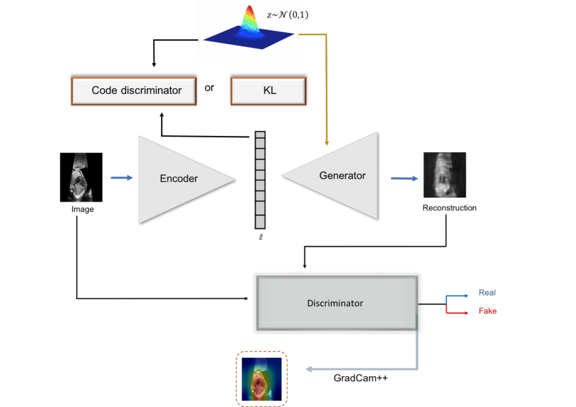
To achieve this, we build a GAN-based model, where the aim of the discriminator networks is to learn the salient features of the fetal images (i.e., heart area) during training. We use an auto-encoding generative adversarial network (-GAN) which makes use of discriminator information in order to predict the anomaly score. -GAN (Rosca et al., 2017)(Kwon et al., 2019) is a fusion of generative adversarial learning (GAN) and a variational autoencoder. It can be considered as autoencoder GAN combining the reconstruction power of an autoencoder with the sampling power of generative adversarial networks. It aims to overcome GAN instabilities during training, which leads to mode collapse while at the same time exploits the advantages of variational autoencoders, producing less blurry images. In -GAN two discriminators focus on the data and latent space respectively. An overview of the proposed architecture is given in Figure 2
Input: fetal ultrasound image , parameter , Number of Epochs:
Output: Models:
We assume a generating process of real fetal cardiac images as and a random prior distribution . Reconstruction, , of an input image is defined as where is a sample from the variational distribution , i.e., . Furthermore, we define as a sample from a normal prior distribution , i.e., .
The encoder () is mapping each real sample from sample space to a point in the latent space , i.e., . It consists of four blocks. Each block contains a Convolutional-Batch Normalisation layer followed by Leaky Rectified Linear Unit (LeakyReLU) activation, down-sampling the resolution of data by two in each block. Spectral Normalisation (Miyato et al., 2018), (Zhang et al., 2019) a weight normalisation method, is used after each convolutional layer. In the last block, after the convolutional layer, an attention gate is introduced (Schlemper et al., 2019), (Zhang et al., 2019). The final layer of the encoder is a tangent layer. The dimension of the latent space is equal to .
The generator synthesises images from latent space back to the sample space , i.e., . The generator regenerates the initial image using four consecutive blocks of transposed convolution-batch normalisation-Rectified Linear Unit (ReLU) activation layers. The last layer is a Hyperbolic tangent (tanh) activation. Similar to encoder spectral normalisation, attention gate layers are used.
The discriminator () takes as input an image and tries to discriminate between real and fake images. The output of the discriminator is a probability for the input being a real or fake image. It consists of four blocks. Each block consists of Convolutional-Batch Normalisation-RELU layers. The last layer is a sigmoid layer. The discriminator treats as real images while the reconstruction from the encoder and samples from , are considered as fake.
A latent discriminator is introduced in order to discriminate latent representations which are generated by the encoder network from samples of a standard Gaussian distribution. The latent code discriminator () consists of four linear layers followed by a Leaky RELU activation. We randomly initialise the encoder, generator and latent code discriminator. The weights for the discriminator are initialised with a normal distribution . We train the architecture by first updating the encoder parameters by minimizing:
| (1) |
We define the generator loss as:
| (2) |
Since we consider encoder and generator as one network the loss for the encoder-generator is:
| (3) |
where and are defined in Eqs. 1 and 2 respectively. The generator is updating twice compared to the encoder in order to stabilize the training procedure.
Then we minimise discriminator loss
| (4) |
Finally, we update the weights of latent code discriminator using
| (5) |
For the learning rate , we use value of after grid search.
The training process of the -GAN model is described in algorithm 1. The networks are trained using the Adam optimizer. Encoder and Generator use the same learning rate, . The same learning rate is also utilised for discriminator and latent code discriminator.
We additionally replace the latent discriminator with an approximation of KL divergence. For a latent vector of dimension we define KL divergence as (Ulyanov et al., 2018):
where and is the mean and standard deviation of each component of the dimensional latent space. Performance in this configuration is subpar, thus we limit the discussion to results with the latent code discriminator.
Furthermore, we apply an analytic estimation of KL divergence using a one-class variational autoencoder (VAE-GAN) similar to (Baur et al., 2018) (Dosovitskiy and Brox, 2016). The VAE-GAN is trained using reconstruction error plus the KL divergence between the latent space () and the normal distribution . For training the VAE-GAN, we first update the encoder and decoder networks as following:
Finally, the discriminator is trained based on the:
where , are set to and respectively after grid search.
A ResNet18 (He et al., 2016)-based architecture encoder and decoder/generator are utilised (with random initialisation). In the ResNet18 encoder/decoder architecture each layer consists of residual blocks and each block is layer deep. We use the same discriminator as in -GAN.
The dimensions of the latent space are . since we use the norm (i.e., mean square error).
All networks are implemented in Python using Pytorch, on a workstation with a NVIDIA Titan X GPU.
3.1 Anomaly detection score
In order to predict an anomaly score , three different strategies are utilised. For an unseen image and its reconstructed image , we utilise as baseline the reconstruction error which is defined as the norm, i.e., between image and reconstructed image (residual).
The second candidate for is the output of the discriminator. should give high scores for reconstructions of original, normal images, but low scores for abnormal images, . Finally, we compute an anomaly score using a gradient-based method, GradCam++, (Chattopadhay et al., 2018). Inspired by (Kimura et al., 2020) (Venkataramanan et al., 2019) (Liu et al., 2020) we apply GradCam++ to the score of the discriminator with regards to the last rectified convolutional layer of the discriminator. This produces attention maps and is also valuable for the localisation of the pathology. The intuition of using attention maps for computing anomaly scores, is based on the hypothesis that after training the discriminator not only learns to discriminate between normal and abnormal samples but also learns to focus on relevant features in the image. Thus, specifically for HLHS, where the left artery is missing or is occluded compared to normal samples, a discriminator should identify and locate this difference. The GradCam++ is computed following:
Let be the logits of the last layer as they are derived from the discriminator network . For the same operators and applied to the feature map we compute weights:
| (6) |
where the gradient weights can be computed as:
| (7) |
and the saliency map (SM) is computed as a linear combination of the forward activation maps followed by a ReLU layer:
| (8) |
We then computed the sum of the attention maps of image and its reconstruction from the Generator network, :
| (9) |
and finally computed the anomaly score as
| (10) |
To compute the anomaly score we encapsulate the information of reconstruction (Kimura et al., 2020). Reconstruction of a normal image should be crisper compared to reconstructions from an anomalous observation. Finally, we attempt to combine anomaly scores, such as with . However, the anomaly detection performance does not improve noteworthily.
3.2 Data
The available dataset contains 2D ultrasound images of four-chamber cardiac views. These are standard diagnostic views according to (NHS, 2015). The images contain labelled examples from normal fetal hearts and hearts with Hypoplastic Left Heart Syndrome (HLHS) (HLHS, 2019) from the same clinic, using exclusively an Aplio i800 GI system for both groups to avoid systematic domain differences. HLHS is a birth defect that affects normal blood flow through the heart. It affects a number of structures on the left side of the heart that do not fully develop.
Our dataset consists of 4-chamber view images for which cases are normal and are abnormal cases. Healthy control view planes have been automatically extracted from examination screen capture videos using a Sononet network (Baumgartner et al., 2017) and manual cleaning from visually trivial classification errors. A set of HLHS view planes that would resemble a 4-chamber view in healthy subjects has been extracted with the same automated Sononet pipeline. Another set has been manually extracted from the examination videos by a fetal cardiologist and 38 cases that are not within 19+0 - 20+6 weeks or show a mix of pathologies have been rejected.
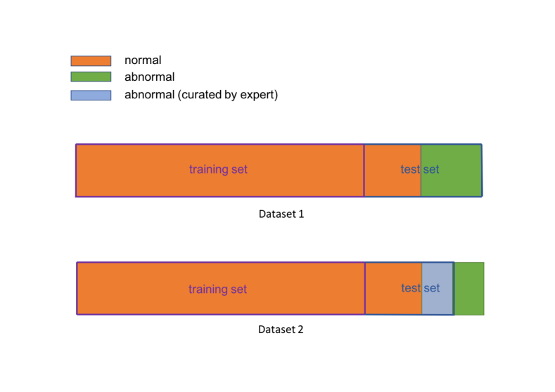
For training, 4-chamber view images, which are considered as normal cases are used. During training, only images from normal fetuses are used. For testing, two different datasets are derived for three different testing scenarios:
For (Figure 2) we use 4-chamber views from all available HLHS cases, extracted by Sononet and cleaned from gross classification errors; in total cases. Further normal cases have been randomly selected from the remaining test split of the healthy controls and added to this dataset. HLHS cases are challenging for Sononet, which has been trained only on healthy views. Thus, in HLHS cases, it will only select views that are close to the feature distribution of healthy 4-chamber views, which are not necessarily the views a clinician would have chosen. For (Figure 2), we use the normal cases from and the expert-curated HLHS images from the remaining, nonexcluded cases. For each of these cases to different view planes have been identified as clinically conclusive. With this dataset we perform two different subject-level experiments: a) selecting one of the four frames randomly and b) using all of the 177 clinically selected views in these 53 subjects and fusing the individual abnormality scores to gain a subject-level assessment. We also evaluate per-frame anomaly results.
The images are rescaled to and normalised to a value range. No image augmentation is used.
4 Evaluation and Results
We evaluate our algorithm both quantitatively as well as qualitatively. The capability of the proposed method to localise the pathology is also examined.
4.1 Quantitative analysis
For evaluation purposes, the anomaly score is computed as described in Section 3.1. For -GAN and VAE-GAN we use , and as anomaly scores as they are presented in Section 3.1.
For comparison with the state-of-the-art we train four algorithms: convolutional autoencoder (CAE) (Makhzani and Frey, 2015; Masci et al., 2011), One-class Deep Support Vector Data Description (DeepSVDD) (Ruff et al., 2018) and f-AnoGAN (Schlegl et al., 2019).
Deep Convolutional autoencoder (DCAE) (Makhzani and Frey, 2015; Masci et al., 2011) is also trained as a baseline. For training, MSE loss is utilised. For DCAE and One-class DeepSVDD we use the same architectures as the ones used for the CIFAR10 dataset in the original work (Ruff et al., 2018). Reconstruction error, i.e., , is defined as anomaly score ().
Deep Support Vector Data Description (DeepSVDD) (Ruff et al., 2018) computes the hypersphere of minimum volume that contains every point in the training set. By minimising the sphere’s volume, the chance of including points that do not belong to the target class distribution is minimised. Since in our case all the training data belongs to one class (negative class-healthy data) we focus on (Ruff et al., 2018) . Let be the network function of the deep neural network with layers and the weights’s parameters of the layer. We denote the center of the hypersphere as . The objective of the network is to minimize the loss which is defined as:
The center is set to be the mean of outputs which is obtained at the initial forward pass. The anomaly score () is then defined at inference stage as the distance between a new test sample to the center of the hyper-sphere, i.e.,
f-AnoGAN (Schlegl et al., 2019) is described in Section 2.2. We were not able to successfully train f-AnoGAN using the same networks as we used for -GAN, hence we utilise similar networks and an identical training framework as described in (Schlegl et al., 2019). We follow the training procedure for the encoder network. As anomaly detection score () a combination of residual loss between the image and its reconstruction and the norm of the discriminator’s features of an intermediate layer is utilised as it is defined in Table 1.
In all algorithms the latent dimension is chosen as . We run all experiments times using different random seeds (Mario Lucic et al., 2018). We report the average precision, recall at the Youden index of the receiver operating characteristic (ROC) curves as well as the average corresponding area under curve (AUC) of the runs of each experiment. Furthermore, we apply the DeLong’s test (DeLong et al., 1988) to obtain z-scores and p-values in order to test how statistically different the AUC curve of the proposed model compared to the corresponding curves of the state-of-the-art models (CAE and DeepSVDD, f-AnoGAN and VAE-GAN) is. We perform four different experiments:
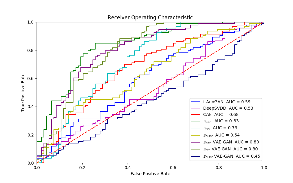
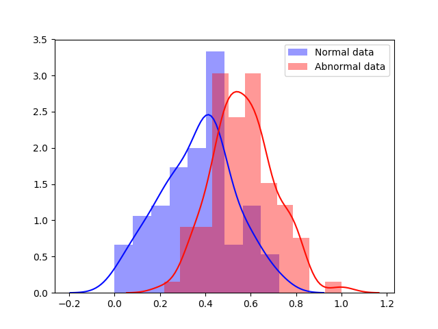
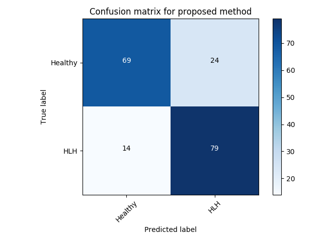
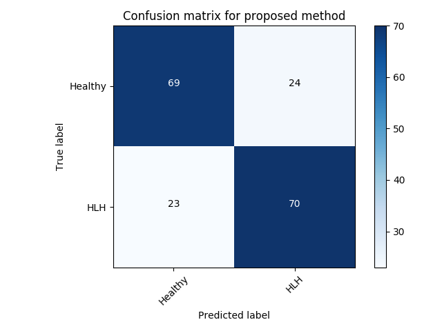
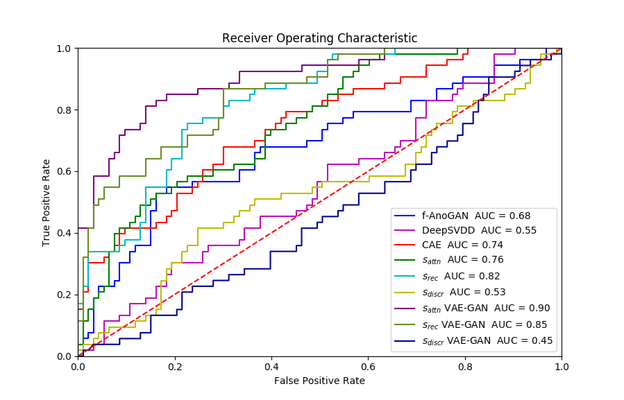
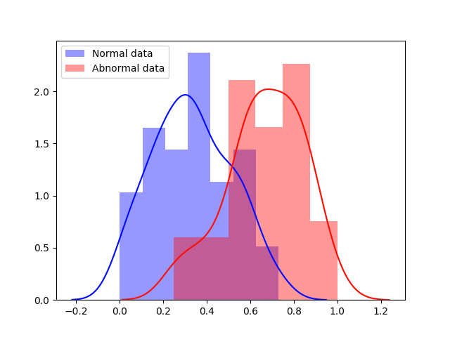
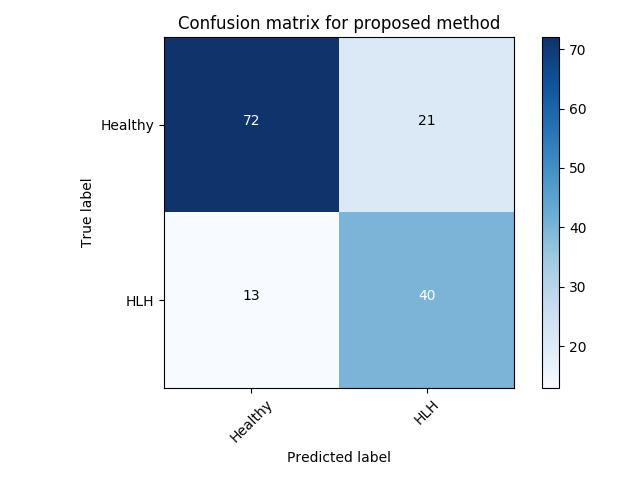
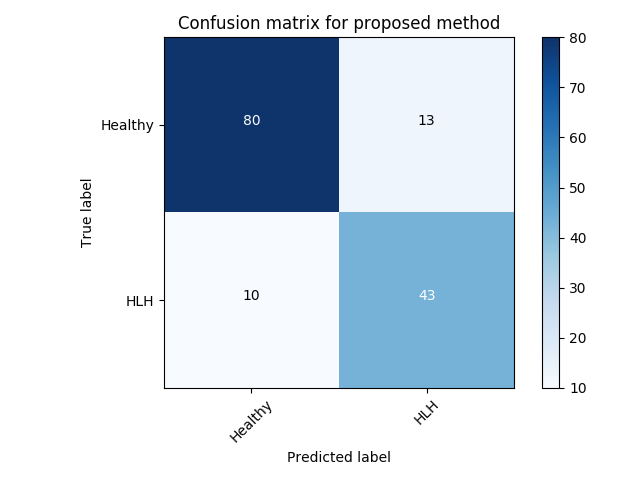
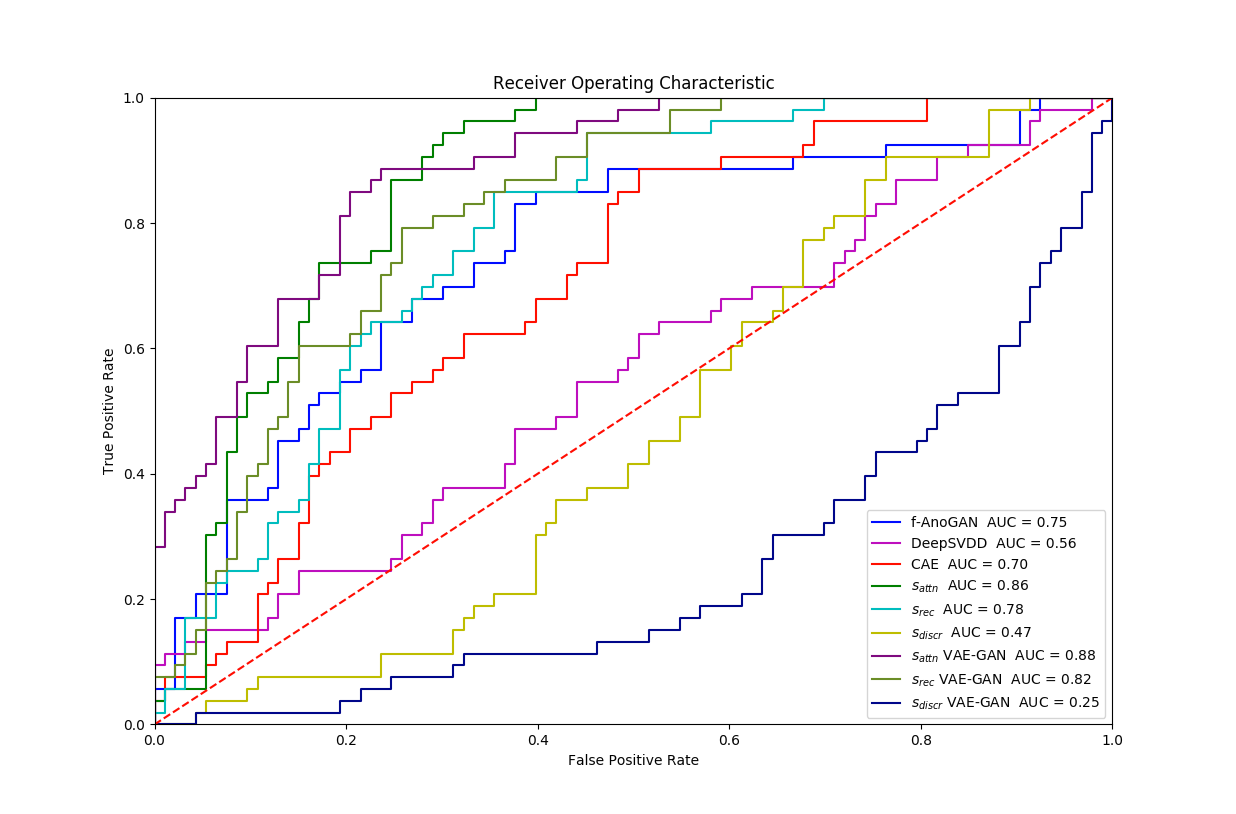
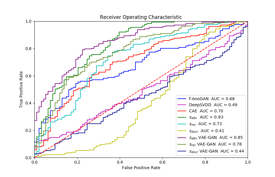
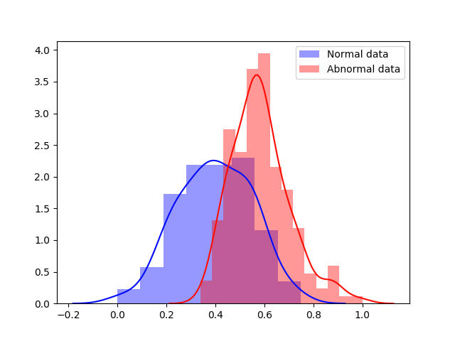
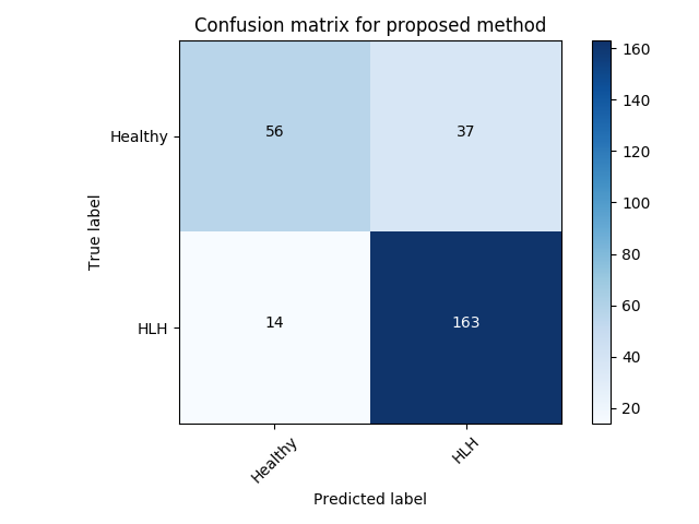
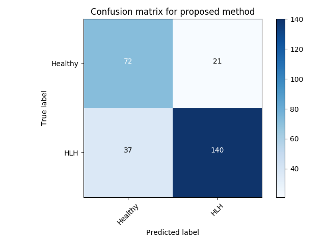
Experiment 1 uses and aims to evaluate general, frame-level outlier detection performance, including erroneous classifications and fetuses below the expected age range. In Table 2, the best performing model based on AUC score is the -GAN method using as anomaly score which achieves an average of AUC. The -GAN model achieves the best precision score. However, regarding F1 score and Recall VAE-GAN outperforms -GAN with and respectively. DeepSVDD shows the best specificity at . Figure 3 shows the ROC for the best performing (AUC, F1) initialisation and the distribution of normal and abnormal scores for the best model of -GAN at the Youden index. We present confusion matrices for the -GAN and the VAE-GAN models in Figure LABEL:fig:conf and Figure LABEL:fig:confvae. For normal cases both models achieve similar classification performance. However, for identifying abnormal cases -GAN seems to have an advantage.
Based on the DeLong’s test, for Exp. 1, for the average scores (of five experiments), -GAN compared to f-AnoGAN yields and . Similarly, the values for -GAN compared to CAE are and . Finally, comparing -GAN and DeepSVDD results in and . Since for all comparisons, we can assume that -GAN performs significantly better than the state-of-the-art when applied to fetal cardiac ultrasound screening for HLHS. Comparing -GAN with VAE-GAN the values are and which does not indicate a significant difference between AUC curves. As can be seen from the results, the GAN-based methods achieve better performance for detecting HLHS.
| Quantitative performance scores | |||||
|---|---|---|---|---|---|
| Method | Precision | Recall | Specificity | F1 score | AUC |
| CAE (Ruff et al., 2018) | |||||
| DeepSVDD (Ruff et al., 2018) | |||||
| f-AnoGAN (Schlegl et al., 2019) | |||||
| (VAE-GAN) | |||||
| (VAE-GAN) | |||||
| (VAE-GAN) | |||||
| (-GAN) | |||||
| (-GAN) | |||||
| (-GAN) | |||||
Experiment 2 uses for specific disease detection capabilities with expert-curated, clinically conclusive 4-chamber views for 53 HLHS cases. We choose one of the relevant views per subject randomly. Table 3 summarises these results. VAE-GAN has the highest AUC, F1, precision and specificity scores using as anomaly score. Also, we note from Figure LABEL:fig:conf1 and Figure LABEL:fig:conf11 that the VAE-GAN method misclassified less HLHS cases while achieving better performance for confirming normal cases. Average F1 score is . Figure 4 shows ROC, anomaly score distribution and confusion matrices at the Youden index of this experiment.
| Quantitative performance scores | |||||
|---|---|---|---|---|---|
| Method | Precision | Recall | Specificity | F1 score | AUC |
| CAE (Ruff et al., 2018) | |||||
| DeepSVDD (Ruff et al., 2018) | |||||
| f-AnoGAN (Schlegl et al., 2019) | |||||
| (VAE-GAN) | |||||
| (VAE-GAN) | |||||
| (VAE-GAN) | |||||
| (-GAN) | |||||
| (-GAN) | |||||
| (-GAN) | |||||
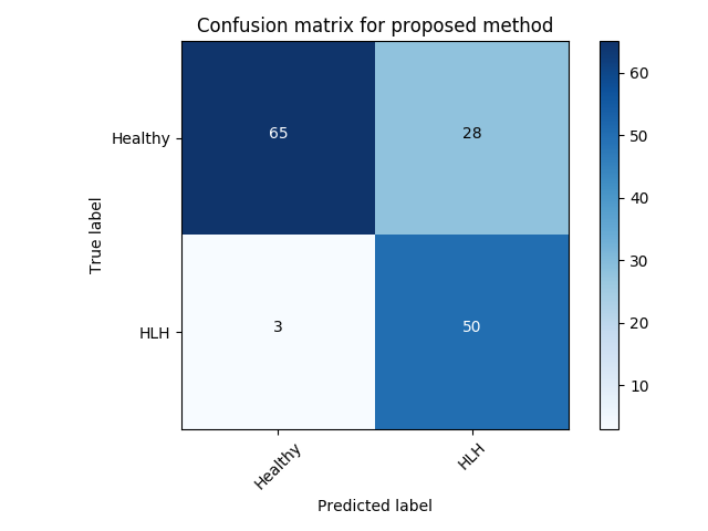
Experiment 3 uses and is similar to Exp. 2 except that we take all clinically identified views for each subject into account. We average the individual anomaly scores for each frame, depending on the number of frames that are available per subject. VAE-GAN achieves a better AUC score with compared to of -GAN as can be seen in Table 4. However, as can be seen from the confusion matrices (best performing initialisation), -GAN shows a better true positive rate at the cost of a higher number of false positives (Figure LABEL:fig:conf2). This configuration might be preferred in a clinical setting since it reduces the number of missed cases at the cost of a slightly higher number of false referrals.
| Quantitative performance scores | |||||
|---|---|---|---|---|---|
| Method | Precision | Recall | Specificity | F1 score | AUC |
| CAE (Ruff et al., 2018) | |||||
| DeepSVDD (Ruff et al., 2018) | |||||
| f-AnoGAN (Schlegl et al., 2019) | |||||
| (VAE-GAN) | |||||
| (VAE-GAN) | |||||
| (VAE-GAN) | |||||
| (-GAN) | |||||
| (-GAN) | |||||
| (-GAN) | |||||


Experiment 4 is similar with the Exp. 3 except that we evaluate frame-level performance in Table 5. VAE-GAN is again better in terms of precision and AUC performance. However, similar to Exp. 3 -GAN has an advantage when recognising the cases with pathology at a cost of a higher false positive rate.
| Quantitative performance scores | |||||
|---|---|---|---|---|---|
| Method | Precision | Recall | Specificity | F1 score | AUC |
| CAE (Ruff et al., 2018) | |||||
| DeepSVDD (Ruff et al., 2018) | |||||
| f-AnoGAN (Schlegl et al., 2019) | |||||
| (VAE-GAN) | |||||
| (VAE-GAN) | |||||
| (VAE-GAN) | |||||
| (-GAN) | |||||
| (-GAN) | |||||
| (-GAN) | |||||
4.2 Qualitative analysis
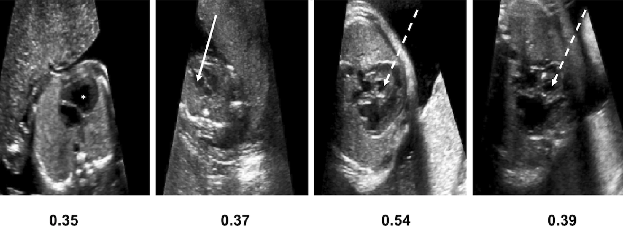
In order to evaluate the ability of the algorithm to localise anomalies, we plot the class activation maps as they are derived from the proposed model. We present results from abnormal cases in (Exp.1) Figure 7. In the abnormal cases, attention focus exactly in the area of heart. As a consequence, anomaly scores in such cases are higher compared to normal cases and correctly indicating the anomalous cases. All anomaly scores are normalised in the range of . There are cases that our algorithm fails to classify correctly. Either they are abnormal and they are classified as normal (False Negative-FN) or they are healthy and identified as anomalous (False Positive-FP). In Figure 8 examples for False Positive cases are presented alongside False Negative cases. Bad image reconstruction quality is a limiting factor. For instance, in some reconstructions either a part of the heart is missing (left or right ventricle/ atrium) or the shape of the heart is quite different from a normal heart (e.g., a very “long” ventricle). As a consequence, not only the reconstruction error is high, but also the attention mechanism focuses in this area, since it is recognised (by the network) as anomalous. Consequently, the total anomaly score is high. In fewer examples the signal-to-noise ratio (SNR) is low, i.e., images are blurry, and so the network fails to reconstruct the images at all. Furthermore, in the False Positive examples Figure 8a, from clinical perspective, the angle is not quite right, so it makes the ventricles look shorter than they are. This confuses the model, forcing the discriminator’s attention to indicate this area as anomalous. Another point which is very interesting to highlight, is that there are cases where some frames are very difficult, even for experts. Such an example is given in Figure 8b, where although the second image from left belongs to an abnormal subject, the specific frame appears normal at the first glance. Such cases also highlight limitations of single-view approaches. In practice, all relevant frames showing the four chamber view could be processed with our method and a majority vote could regarding referral be calibrated on a ROC curve.
All the above plots and comparisons utilise the top- performing experiment among all the runs of the experiments for -GAN.
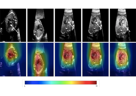
*= dominant RV with no visible LV cavity, solid white arrow = deceptively normal-looking LV, dashed white arrow = globular, hypoplastic LV

5 Discussion
Our results are promising and confirm that automated anomaly detection can work in fetal 2D ultrasound as shown on the example of HLHS. For this pathology we achieve an average accuracy of AUC, improving significantly the detection rate of front-line-of-care sonographers during screening, which is often below 60% (Chew et al., 2007). However, there are open issues.
False negative rates are critical for clinical diagnosis and downstream treatment. In a clinical setting, a method with zero false negative predictions would be preferred, i.e., a method that never misses an anomaly, but potentially predicts a few false positives. Assuming that the false positive rate of such an algorithm is significantly below the status quo, the benefits for antenatal detection and potentially better postnatal outcomes would outweigh the costs. Of course, an algorithm with a 100% false positive rate is also not desirable, hence calibration on the ROC must be performed.
A key aspect of the proposed algorithm is the ability of the discriminator to highlight decisive areas in images. In order to achieve this, it is necessary to produce good reconstructions of normal images. However, reconstruction quality can be limited, depending on the given sample. A larger dataset could provide a mitigation strategy for this. Furthermore, alternative ways for visualising attention could be explored for disease-specific applications such as implicit mechanisms of attention like attention gates (Schlemper et al., 2019).
Although we have experimented with different type of noise (e.g Uniform) and various augmentation techniques (e.g horizontal flip, intensity changes) we did not notice an improvement in anomaly detection performance. However, a further investigation of other augmentation techniques should be done.
Moreover, it would be interesting to explore the sensitivity of our method for other sub-types of congenital heart disease. Intuitively, accuracy of a general anomaly detection method should be similarly high for other syndromes that affect the morphological appearance of the fetal four-chamber view. HLHS has a particularly grossly abnormal appearance. There are a lot of other CHD examples with a subtly abnormal four chamber view that would probably be much harder to detect even for human experts. Additionally, in practice, confounding factors may bias anomaly detection methods towards more obvious outliers, while subtle signs of disease or indicators encoded in other dimensions like the spatio-temporal domain may still be missed.
Finally, robust time-series analysis is still a challenging fundamental research question and we are looking forward to extending our method to full video sequences in future work.
6 Conclusion
In this paper we attempt to consider the detection of congenital heart disease as a one-class anomaly detection problem, learning only from normal samples. The proposed unsupervised architecture shows promising results and achieves better performance compared to existing state-of-the-art image anomaly detection methods. However, since clinical practice requires highly reliable anomaly detection methods, more work will need to be done to avoid false positives to mitigate patient stress and strain on healthcare systems and false negatives to prevent missed diagnoses.
Acknowledgements
EC was supported by an EPSRC DTP award. TD was supported by an NIHR Doctoral Fellowship. We thank the volunteers and sonographers from routine fetal screening at St. Thomas’ Hospital London. This work was supported by the Wellcome Trust IEH Award [102431] for the Intelligent Fetal Imaging and Diagnosis project (www.ifindproject.com) and EPSRC EP/S013687/1. The study has been granted NHS R&D and ethics approval, NRES ref no = 14/LO/1086. The research was funded/supported by the National Institute for Health Research (NIHR) Biomedical Research Center based at Guy’s and St Thomas’ NHS Foundation Trust, King’s College London and the NIHR Clinical Research Facility (CRF) at Guy’s and St Thomas’. Data access only in line with the informed consent of the participants, subject to approval by the project ethics board and under a formal Data Sharing Agreement. The views expressed are those of the author(s) and not necessarily those of the NHS, the NIHR or the Department of Health.
References
- Arjovsky et al. (2017) M. Arjovsky, S. Chintala, and L. Bottou. Wasserstein GAN. arXiv preprint arXiv:1701.07875, 2017.
- Arnaout et al. (2020) R. Arnaout, L. Curran, Y. Zhao, J. Levine, E. Chinn, and A. Moon-Grady. Expert-level prenatal detection of complex congenital heart disease from screening ultrasound using deep learning. medRxiv, 2020. doi: 10.1101/2020.06.22.20137786.
- Baumgartner et al. (2017) C F. Baumgartner, K. Kamnitsas, J. Matthew, T. P. Fletcher, S. Smith, L M. Koch, B. Kainz, and D. Rueckert. Sononet: Real-time detection and localisation of fetal standard scan planes in freehand ultrasound. IEEE Trans. Medical Imaging, 36(11):2204–2215, 2017.
- Baur et al. (2018) C. Baur, B. Wiestler, S. Albarqouni, and N. Navab. Deep autoencoding models for unsupervised anomaly segmentation in brain mr images. International MICCAI Brainlesion Workshop, pages 161–169, 2018.
- Bennasar et al. (2010) M. Bennasar, J.M Martínez, O. Gómez, J. Bartrons, A. Olivella, B. Puerto, and E. Gratacós. Accuracy of four-dimensional spatiotemporal image correlation echocardiography in the prenatal diagnosis of congenital heart defects. Ultrasound in Obstetrics and Gynecology, 36(4), pages 458–464, 2010.
- Chattopadhay et al. (2018) A. Chattopadhay, A. Sarkar, P. Howlader, and V. N. Balasubramanian. Grad-CAM++: Generalized Gradient-Based Visual Explanations for Deep Convolutional Networks. 2018 IEEE Winter Conference on Applications of Computer Vision (WACV), pages 839–847, 2018.
- Chew et al. (2007) C Chew, JL Halliday, MM Riley, and DJ Penny. Population-based study of antenatal detection of congenital heart disease by ultrasound examination. Ultrasound in Obstetrics and Gynecology: The Official Journal of the International Society of Ultrasound in Obstetrics and Gynecology, 29(6):619–624, 2007.
- DeLong et al. (1988) E.R DeLong, D.M DeLong, and D.L Clarke-Pearson. Comparing the areas under two or more correlated receiver operating characteristic curves: a nonparametric approach. Biometrics, 44(3):837–845, 1988. doi: 10.2307/2531595.
- Dosovitskiy and Brox (2016) A. Dosovitskiy and T. Brox. Generating images with perceptual similarity metrics based on deep networks. Advances in Neural Information Processing Systems 29 (NIPS), 29, 2016.
- Gong et al. (2020) Y. Gong, Y. Zhang, H. Zhu, J. Lv, H. Cheng, Q. Zhang, Y. He, and S. Wang. Fetal congenital heart disease echocardiogram screening based on dgacnn: Adversarial one-class classification combined with video transfer learning. IEEE Transactions on Medical Imaging, 39(4):1206–1222, 2020.
- Gulrajani et al. (2017) I. Gulrajani, F. Ahmed, M. Arjovsky, V. Dumoulin, and AC. Courville. Improved training of Wasserstein GANs. arXiv preprint arXiv:1704.00028, 2017.
- He et al. (2016) K. He, X. Zhang, S. Ren, and J. Sun. Deep residual learning for image recognition. In proceedings of the IEEE conference on computer vision and pattern recognition, pages 770–778, 2016.
- HLHS (2019) HLHS. Facts about Hypoplastic Left Heart Syndrome, National Center on Birth Defects and Developmental Disabilities, Centers for Disease Control and Prevention. https://www.cdc.gov/ncbddd/heartdefects/hlhs.html, 2019.
- (14) B. J. Holland, J. A. Myers, and C. R. Woods Jr. Prenatal diagnosis of critical congenital heart disease reduces risk of death from cardiovascular compromise prior to planned neonatal cardiac surgery: a meta-analysis. Ultrasound in Obstetrics and Gynecology, 45:631 – 638.
- Isola et al. (2017) P. Isola, J-H. Zhu, T. Zhou, and AA. Efros. Image-to-image translation with conditional adversarial networks. CVPR, 2017.
- Kimura et al. (2020) D. Kimura, S. Chaudhury, M. Narita, A. Munawar, and R. Tachibana. Adversarial Discriminative Attention for Robust Anomaly Detection. IEEE Winter Conference on Applications of Computer Vision, WACV, pages 2161–2170, 2020.
- Kwon et al. (2019) G. Kwon, C. Han, and R.V Daeshik. Generation of 3D Brain MRI Using Auto-Encoding Generative Adversarial Networks. Medical Image Computing and Computer Assisted Intervention - MICCAI 2019 - 22nd International Conference, Shenzhen, China, October 13-17, 2019, Proceedings, Part III, pages 118–126, 2019. doi: 10.1007/978-3-030-32248-9\_14.
- Liu et al. (2020) W. Liu, R. Li, M. Zheng, S. Karanam, Z. Wu, B. Bhanu, R.J Radke, and O.I Camps. Towards Visually Explaining Variational Autoencoders. 2020 IEEE/CVF Conference on Computer Vision and Pattern Recognition, CVPR 2020, Seattle, WA, USA, June 13-19, 2020, pages 8639–8648, 2020. doi: 10.1109/CVPR42600.2020.00867.
- Makhzani and Frey (2015) A. Makhzani and B.J Frey. Winner-take-all autoencoders. Advances in Neural Information Processing Systems 28: Annual Conference on Neural Information Processing Systems 2015, December 7-12, 2015, Montreal, Quebec, Canada, pages 2791–2799, 2015.
- Mario Lucic et al. (2018) M. Mario Lucic, K. Kurach, M. Michalski, S. Gelly, and O. Bousquet. Are GANs Created Equal? A Large-Scale Study. Advances in Neural Information Processing Systems 31: Annual Conference on Neural Information Processing Systems, pages 698–707, 2018.
- Masci et al. (2011) J. Masci, U. Ueli Meier, D. C. Dan C. Ciresan, and J. Schmidhuber. Stacked convolutional auto-encoders for hierarchical feature extraction. Artificial Neural Networks and Machine Learning - ICANN 2011 - 21st International Conference on Artificial Neural Networks, Espoo, Finland, June 14-17, 2011, Proceedings, Part I, pages 52–59, 2011.
- Miyato et al. (2018) T. Miyato, T. Kataoka, M. Koyama, and Y. Yoshida. Spectral Normalization for Generative Adversarial Networks. 6th International Conference on Learning Representations, ICLR 2018, Vancouver, BC, Canada, April 30 - May 3, 2018, Conference Track Proceedings, 2018.
- Ngo et al. (2019) CP. Ngo, AA. Winarto, Khor Li Kou C., S. Park, F. Akram, and HK. Lee. Fence GAN: Towards Better Anomaly Detection. arXiv preprint arXiv:1904.01209, 2019.
- NHS (2015) NHS. Fetal anomaly screening programme: programme handbook June 2015. Public Health England, 2015.
- Oza and Patel (2019) P. Oza and V. M. Patel. One-class convolutional neural network. IEEE Signal Processing Letters, 26:277–281, 2019.
- Perera et al. (2019) P. Perera, R. Nallapati, and B. Xiang. Ocgan: One-class novelty detection using gans with constrained latent representations. IEEE Conference on Computer Vision and Pattern Recognition, CVPR, pages 2898–2906, 2019.
- Perera et al. (2021) P. Perera, P. Oza, and V. M. Patel. One-class classification: A survey. CoRR, arXiv:2101.03064, 2021.
- Petersen et al. (2013) Steffen E Petersen, Paul M Matthews, Fabian Bamberg, David A Bluemke, Jane M Francis, Matthias G Friedrich, Paul Leeson, Eike Nagel, Sven Plein, Frank E Rademakers, et al. Imaging in population science: cardiovascular magnetic resonance in 100,000 participants of uk biobank-rationale, challenges and approaches. Journal of Cardiovascular Magnetic Resonance, 15(1):46, 2013.
- Pidhorskyi et al. (2018) S. Pidhorskyi, R. Almohsen, and G. Doretto. Generative probabilistic novelty detection with adversarial autoencoders. Advances in neural information processing systems, pages 6822–6833, 2018.
- Pinto et al. (2012) NM. Pinto, HT. Keenan, LL. Minich, MD. Puchalski, M. Heywood, and LD. Botto. Barriers to prenatal detection of congenital heart disease: a population-based study. Ultrasound in Obstetrics and Gynecology, 40(4),, pages 418–425, 2012.
- Radford et al. (2016) A. Radford, L. Metz, and S Chintala. Unsupervised representation learning with deep convolutional generative adversarial networks. 4th International Conference on Learning Representations, ICLR 2016,San Juan, Puerto Rico, May 2-4, 2016, Conference Track Proceedings, 2016.
- Rosca et al. (2017) M. Rosca, B. Lakshminarayanan, D. Warde-Farley, and S. Mohamed. Variational Approaches for Auto-Encoding Generative Adversarial Networks. arXiv preprint arXiv:1706.04987, 2017.
- Ruff et al. (2018) L. Ruff, R. Vandermeulen, N. Goernitz, L. Deecke, S. A. Siddiqui, A. Binder, E. Müller, and M. Kloft. Deep One-Class Classification. Proceedings of Machine Learning Research, pages 4393–4402, 2018.
- Sabokrou et al. (2018) M. Sabokrou, M. Khalooei, M. Fathy, and E. Adeli. Adversarially Learned One-Class Classifier for Novelty Detection. 2018 IEEE Conference on Computer Vision and Pattern Recognition, CVPR 2018, Salt Lake City, UT, USA, June 18-22, 2018, pages 3379–3388, 2018.
- Schlegl et al. (2017) T. Schlegl, P. Seeböck, SM. Waldstein, U. Schmidt-Erfurth, and G. Langs. Unsupervised Anomaly Detection with Generative Adversarial Network to Guide Marker Discovery. Information Processing in Medical Imaging - 25th International Conference, IPMI 2017, Boone, NC, USA, June 25-30, 2017, Proceedings, pages 146–157, 2017. doi: 10.1007/978-3-319-59050-9\_12.
- Schlegl et al. (2019) T. Schlegl, P. Seeböck, SM. Waldstein, G Langs, and U.. Schmidt-Erfurth. f-AnoGAN: Fast unsupervised anomaly detection with generative adversarial networks. Medical Image Analysis, pages 30–44, 2019. doi: 10.1016/j.media.2019.01.010.
- Schlemper et al. (2019) J. Schlemper, O. Oktay, M. Schaap, M. Heinrich, B. Kainz, B. Glocker, and D. Rueckert. Attention gated networks: Learning to leverage salient regions in medical images. Medical Image Analysis, pages 197 – 207, 2019. doi: https://doi.org/10.1016/j.media.2019.01.012.
- Schölkopf et al. (2001) B. Schölkopf, J. C. Platt, J. C. Shawe-Taylor, A. J. Smola, and R. C. Williamson. Estimating the support of a high-dimensional distribution. Neural Computation, 13:1443–1471, 2001.
- Shen et al. (2020) H. Shen, J. Chen, R. Wang, and J. Zhang. Counterfeit Anomaly Using Generative Adversarial Network for Anomaly Detection. IEEE Access, pages 133051–133062, 2020.
- Tax and Duin (2004) D.M.J Tax and R.P.W Duin. Support vector data description. Machine Learning, 54:45–66, 2004.
- Ulyanov et al. (2018) D. Ulyanov, A. Vedaldi, and V. S. Lempitsky. It takes (only) two: Adversarial generator-encoder networks. AAAI, 2018.
- van Velzen et al. (2016) CL. van Velzen, SA. Clur, MEB. Rijlaarsdam, CJ. Bax, E. Pajkrt, MW. Heymans, MN. Bekker, J. Hruda, CJM. de Groot, NA. Blom, and MC. Haak. Prenatal detection of congenital heart disease–results of a national screening programme. BJOG: An international journal in Obstetrics and Gynaecology , 123(3), pages 400–407, 2016.
- Venkataramanan et al. (2019) S. Venkataramanan, K-C. Peng, R.V. Singh, and A. Mahalanobis. Adversarial Discriminative Attention for Robust Anomaly Detection. arXiv preprint arXiv:1911.08616, 2019.
- Yeo et al. (2018) L. Yeo, S. Luewan, and R. Romero. Fetal Intelligent Navigation Echocardiography (FINE) detects of Congenital Heart Disease. Journal of ultrasound in medicine, 37(11),, page 2577–2593, 2018.
- Zaheer et al. (2020) M. Z. Zaheer, J.-h Lee, M. Astrid, and S-I Lee. Old is gold: Redefining the adversarially learned one-class classifier training paradigm. Proceedings of the IEEE/CVF Conference on Computer Vision and Pattern Recognition, pages 14183–14193, 2020.
- Zhang et al. (2019) H. Zhang, I. J Goodfellow, D.N Metaxas, and A. Odena. Self-attention generative adversarial networks. Proceedings of the 36th International Conference on Machine Learning, ICML 2019, 9-15 June 2019, Long Beach, California, USA, 97:7354–7363, 2019.
- Zhou et al. (2020) K. Zhou, S. Gao, J. Cheng, Z. Gu, H. Fu, Z. Tu, J. Yang, Y. Zhao, and J. Liu. Sparse-Gan: Sparsity-Constrained Generative Adversarial Network for Anomaly Detection in Retinal OCT Image. 17th IEEE International Symposium on Biomedical Imaging, ISBI 2020, Iowa City, IA, USA, April 3-7, 2020, pages 1227–1231, 2020.