

1 Introduction
Anatomical landmark localization is an important topic in medical image analysis, e.g., as a preprocessing step for segmentation (Beichel et al., 2005; Heimann and Meinzer, 2009; Štern et al., 2011), registration (Johnson and Christensen, 2002; Urschler et al., 2006), as well as for deriving surgical or diagnostic measures like the location of bones in the hip (Bier et al., 2019), curvature of the spine (Vrtovec et al., 2009), bone age estimation (Štern et al., 2019), or misalignment of teeth or the jaw (Wang et al., 2016). Unfortunately, anatomical landmarks can be difficult to define unambiguously, especially for landmarks that do not lie on distinct anatomical structures like the tip of the incisor, but on smooth edges like the tip of the chin. Ambiguity in defined landmark positions leads to difficulty in annotation which is reflected not only in a large inter-observer variability between different annotators, but also in a large intra-observer variability that is dependent on the daily constitution of a single annotator. Due to this uncertainty, a machine learning predictor that has been trained on potentially ambiguous annotations should model landmarks not only as single locations, but rather as distributions over possible locations. Taking the inconsistencies introduced by intra- and inter-observer variability of the annotators into account during decision making will lead to a potential improvement in clinical workflow and patient treatment (Lindner et al., 2016). Furthermore, estimating the uncertainty that reflects the annotation ambiguities helps interpreting the output of machine learning based prediction software (Gal and Ghahramani, 2016), which is especially useful in the medical imaging domain (Wang et al., 2019b; Nair et al., 2020; Wickstrøm et al., 2020) where explainability is crucial (Gunning et al., 2019).
1.1 Contributions
Differently from state-of-the-art methods that use heatmap based regression for predicting single landmark locations, in this work we show that heatmaps can also be used to estimate the landmark uncertainty caused by annotation ambiguities. To this end, we first adapt the heatmap regression framework to allow optimization of not only the model parameters of the network but also the shape parameters of the target heatmaps. By doing so, we model the uncertainty based on annotation ambiguities of the entire training dataset, representing a homoscedastic aleatoric uncertainty that is the same for each image in the dataset. We name this uncertainty dataset-based annotation uncertainty. Second, during inference, a Gaussian function is fitted to the predicted heatmap to not only predict the most probable landmark location but its distribution, i.e., a heteroscedastic aleatoric uncertainty that is specific for each image. We name this uncertainty sample-based annotation uncertainty. We evaluate our approach on two datasets, i.e., on left hand radiographs and lateral cephalograms, showing that the uncertainties correlate with the magnitude and direction of the average localization error as well as the inter-observer variabilities.
This work extends our MICCAI-UNSURE 2020 workshop paper (Payer et al., 2020) in the following: (1) We improved the representativeness of the inter-observer variability used in our experiments by extending the annotation of the cephalogram dataset with additional annotations from nine observers. (2) We performed an in-depth analysis of our proposed method for estimating the dataset-based and sample-based annotation uncertainty on the newly annotated dataset. (3) We introduced a new experiment showing the importance of utilizing landmark location uncertainty into decision making with an example of measuring anatomical abnormalities in lateral cephalograms. (4) Finally, we included more details of the method, and extended our literature review and discussion section.
2 Related Work
2.1 Landmark Localization
Due to the variable visual appearance of the anatomy defining a landmark position in images, modern methods for landmark localization are based on convolutional neural networks (CNNs) because of their superior image feature extraction capabilities as compared to other machine learning techniques (Toshev and Szegedy, 2014; Tompson et al., 2014; Wei et al., 2016; Payer et al., 2016; Newell et al., 2016; Yang et al., 2017; Payer et al., 2019; Bier et al., 2019). While earlier work that applied CNNs for human pose estmation – a task similar to anatomical landmark localization – uses CNNs for directly regressing landmark coordinates (Toshev and Szegedy, 2014), more recent methods for human pose estimation apply CNNs with the heatmap regression framework (Tompson et al., 2014; Wei et al., 2016; Newell et al., 2016). In the heatmap regression framework, the network is trained not to directly predict the landmark coordinates, but a heatmap which is generated as an image of a Gaussian function centered at the coordinate of the landmark. Thus, in this image-to-image mapping, the network learns to generate high responses on locations close to the target landmarks, while responses on wrong locations are being suppressed.
In our previous work (Payer et al., 2016), we introduced the CNN-based heatmap regression framework to anatomical landmark localization, while additionally proposing a CNN architecture called SpatialConfiguration-Net (SCN), which integrates spatial information of landmarks directly into an end-to-end trained, fully convolutional network. Building upon our approach, Yang et al. (2017) used the heatmap regression framework to generate predictions for landmarks with missing responses and incorporated an additional postprocessing step to remove false-positive responses. Bier et al. (2018) used heatmap regression for localizing landmarks on radiographs of the hips. To cope with the small number of images of their training dataset, they implement a sophisticated image synthesis framework based on projecting three-dimensional volumes to two-dimensional images and pretrain their networks with these synthetic images. Mader et al. (2019) adapted the heatmap regression networks for predicting more than a hundred landmarks on a dataset of spinal CT volumes. However, due to memory restrictions resulting from a large number of landmarks, they do not incorporate upsampling layers, thus reducing the accuracy of their heatmap regression outputs. Other recent methods use a coarse-to-fine approach by combining global and local image information with an attention-guided mechanism (Zhong et al., 2019), or with multiplying intermediate network outputs to restrict local responses to their global position (Chen et al., 2019).
In all aforementioned methods, the size of the target heatmaps, i.e., the variance of the Gaussian function, is fixed for each landmark and needs to be predefined before network training. Although our previous work in Payer et al. (2019) indicated that learning the parameters of an isotropic target Gaussian function for each landmark heatmap independently increases prediction accuracy, we did not provide any interpretation of the estimated heatmap size. Moreover, while there exist work that fits isotropic Gaussian functions to the predicted heatmap outputs for obtaining a more robust point prediction, e.g., Liu et al. (2019), most methods only take the single point-wise coordinate prediction as a final output and are not considering the remaining information in the heatmap prediction. Thus, to the best of our knowledge, none of the methods has investigated how the target Gaussian functions or the Gaussian function fitted to the heatmap prediction correlates with the uncertainty of landmark localization.
2.2 Uncertainty Estimation
Uncertainty estimation in medical imaging has been widely adopted and used in segmentation, e.g., for segmenting multiple sclerosis lesions (Nair et al., 2020), the whole-brain (Roy et al., 2018), the fetal brain and brain tumors (Wang et al., 2019a), the carotid artery (Camarasa et al., 2020) as well as for ischemic stroke lesion and vessel extraction from retinal images (Kwon et al., 2020). Furthermore, uncertainty estimation was applied for disease detection using a diabetic retinopathy dataset (Leibig et al., 2017; Ayhan and Berens, 2018), for classification of skin lesions (Mobiny et al., 2019) and for probabilistic classifier-based image registration (Sedghi et al., 2019). A number of uncertainty metrics have been proposed in literature, which can be categorized into model (epistemic) and data (aleatoric) uncertainty (Kendall and Gal, 2017). While epistemic uncertainty represents the prediction confidence of the model for an unseen sample based on its similarity to training data samples, aleatoric uncertainty is caused by the observation noise inherent to the dataset.
Epistemic uncertainty for neural networks involves the use of probabilistic models, where the prediction given an image is not deterministic. This can be achieved with Bayesian Neural Networks (BNN), where weights are not represented as scalars but as distributions. During training, the parameters of the weight distributions are learned, while during inference, the probabilistic output is generated by combining multiple predictions for different weights sampled from the learned distributions (Blundell et al., 2015; Shridhar et al., 2019). A popular approximation of BNNs is Monte Carlo-Dropout (MCD) (Gal and Ghahramani, 2016). Here, the weight distributions are approximated by reusing Dropout (Srivastava et al., 2014) during inference to retrieve a set of stochastic predictions. Since MCD is easy to implement and computationally more efficient than BNNs, it is the most common method to model epistemic uncertainty in medical imaging (Leibig et al., 2017; Roy et al., 2018; Mobiny et al., 2019; Wang et al., 2019a; Camarasa et al., 2020; Kwon et al., 2020; Nair et al., 2020).
Aleatoric uncertainty for neural networks can be estimated by considering network outputs as distributions rather than point predictions. For classification tasks, this can be achieved by using not only the most probable class as the prediction, but the distribution represented by the probabilistic network outputs (Kendall and Gal, 2017). For regression tasks, this can be achieved by adding additional network outputs that model the assumed distribution of the observed annotation noise (Kendall and Gal, 2017; Kwon et al., 2020). For example, when assuming the annotation noise is normally distributed, the network is trained to not only predict the mean but also the variance of the distribution as an additional network output. Aleatoric uncertainty has only recently been investigated in landmark localization for computer vision tasks like pose estimation (Chen et al., 2019; Gundavarapu et al., 2019). Nevertheless, it was only done in the context of occluded landmarks. Due to large inter- and intra-observer variabilities (Chotzoglou and Kainz, 2019; Jungo et al., 2018), the dominant source of aleatoric uncertainty in the medical domain is annotation ambiguity. To the best of our knowledge, there is no previous work that shows how to evaluate annotation uncertainty in medical images from noisy data annotation.
3 Uncertainty Estimation in Landmark Localization
3.1 Heatmap Regression for Dataset-Based Uncertainty
In landmark localization the task is to use an input image with to determine the coordinates of specific landmarks within the extent of the image . In the heatmap regression framework, a CNN with parameters is set up to predict heatmaps , representing the pseudo-probability of the location of landmark . As has been done in several other works (e.g., Tompson et al. (2014); Newell et al. (2016); Payer et al. (2016); Zhong et al. (2019)), a target heatmap for landmark with coordinate can be represented as an isotropic two-dimensional Gaussian function, i.e.,
| (1) |
The mean of the Gaussian is set to the target landmark’s coordinate , while the size of the isotropic Gaussian is defined by . A scaling factor is used to avoid numerical instabilities during training. Fully convolutional networks that predict heatmaps can then be trained with a pixel-wise loss to minimize the difference between predicted heatmaps and target heatmaps for all landmarks by updating the network parameters , i.e.,
| (2) |
Crucial hyperparameters when optimizing the CNN are the sizes of the Gaussian heatmaps, since suboptimal lead to either reduced prediction accuracy or reduced robustness (Payer et al., 2019). All landmark specific can be found via hyperparameter searching techniques (e.g., grid search), however, such approaches are time consuming. Therefore, in our previous work (Payer et al., 2019), sigmas which are unique for each landmark are learned directly during network optimization. Thus, in Payer et al. (2019), we adapted the pixel-wise loss function from Eq. (2) to
| (3) |
Since the parameters of the Gaussian functions are also treated as unknowns, we enable learning them in addition to the network parameters . Thus, the gradient is not only backpropagated through the predicted heatmaps to update the network parameters , but also through the target heatmaps to update the individual target heatmap sizes . The second term in Eq. (3) is used as a regularization to prefer smaller sigma values, as otherwise minimizing the difference between and could lead to the trivial solution where with . It is important to note that although the learned target heatmap sizes are different for each landmark, each target heatmap size is the same for all images in the dataset.
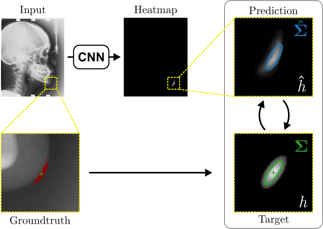
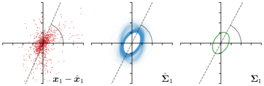
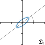
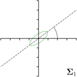
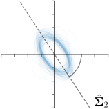
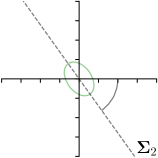
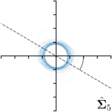
As we will show in our experiments, learning values enables the network to encode the prediction uncertainty for each landmark individually. The more certain the network is in its prediction of a specific landmark, the smaller the target heatmap size will be. However, when using isotropic Gaussian functions as in Eq. (1) as the target heatmaps, information of the directional uncertainty cannot be modeled, which would be beneficial for landmarks that are ambiguous only in a specific direction (see Fig. 1).
In this work, we propose to model the target heatmaps with anisotropic Gaussian functions. A target heatmap is represented as an image of an anisotropic two-dimensional Gaussian function , i.e.,
| (4) |
Differently to Eq. (1), the shape of the Gaussian is not defined by only a single value but by a full covariance matrix . This way, the target heatmaps are able to have an orientation and varying extents in different directions. To separately analyze the orientation and the extent, the covariance matrix can be decomposed into
| (5) |
with
| (6) |
where represents the angle of the Gaussian function’s major axis, and and represent its extent in major and minor axis, respectively.
The final loss function for simultaneously regressing heatmaps is defined as
| (7) |
Same as in Eq. (3), the first term in Eq. (7) minimizes the differences between the predicted heatmaps and the target heatmaps for all landmarks , while we now not only learn the isotropic but all covariance parameters of the Gaussian functions (, , and ). Same as before, the second term of Eq. (3) is used to prefer smaller Gaussian extents by penalizing with factor . Note that while the mean parameters of the Gaussian functions () are set to the groundtruth landmark locations and differ for each training image, the covariance parameters of the target heatmaps are learned for the whole dataset.
Analyzing Eq. (7) in more detail, not only the predicted heatmaps aim to be close to the target heatmaps but also the target heatmaps aim to be close to the predicted heatmaps . For each landmark , and receive feedback from each other during training (see Fig. 1). While the network parameters are updated to better model the shape of the target heatmap , at the same time, the covariance parameters of each target heatmap (, , and ) are updated to better model the shape of the predicted heatmap . Note that, while is learned from a single annotation per image, the CNN sees one annotation for each image in the training set. This allows implicitly modeling the ambiguities of landmark annotations for the whole training dataset representing a dataset-based annotation uncertainty.
3.2 Heatmap Fitting for Sample-Based Uncertainty
As the output of heatmap regression networks are heatmaps that correspond to the landmarks rather than their coordinates, each landmark’s coordinate needs to be obtained from the predicted heatmaps . Previous work often uses the coordinate of the maximum response or the center of mass of the predicted heatmaps as the landmark’s coordinate. However, this represents only the most probable landmark location, but not the whole distribution of possible landmark locations.
As the target heatmaps are modeled as Gaussian functions, the predicted heatmaps are also expected to be Gaussian functions, see Eq. (4). Hence, the distribution of possible landmark locations is captured by fitting Gaussian functions to the predicted heatmaps . We use a robust least squares curve fitting method (Branch et al., 1999) to fit the Gaussian function (see Eq. (4)) to the predicted heatmaps initialized to the respective maximum and obtain the fitted Gaussian parameters and with . As the fitted Gaussian function models the distribution of possible locations, the parameters represent a directional sample-based annotation uncertainty of the landmark location during inference.
4 Experimental Setup
4.1 Networks
SpatialConfiguration-Net for Anatomical Landmark Localization:
Our proposed method to learn anisotropic Gaussian heatmaps can be combined with any image-to-image based network architecture. In this work, the SpatialConfiguration-Net (SCN) by Payer et al. (2019) is used, due to its state-of-the-art performance. We implement learning of Gaussian functions with arbitrary covariance matrices and use the SCN with the default parameters trained for 40,000 iterations. Furthermore, training data augmentation is employed, i.e., random intensity shift and scale as well as translation, scaling, rotation, and elastic deformation. We use weight regularization with a factor of . In Eq. (4) we set ; in Eq. (7), we initialize , , and set .
Monte Carlo-Dropout to Estimate Label Distributions:
To compare to a method for estimating uncertainty, we employ Monte Carlo-Dropout (MCD) by Gal and Ghahramani (2016) to predict a set of different heatmaps per landmark . Two MCD-based approaches are applied to determine the landmark prediction and the covariance parameters :
(1) MCD-,max: In a majority of methods using MCD (Leibig et al., 2017; Roy et al., 2018; Camarasa et al., 2020; Kwon et al., 2020; Nair et al., 2020), the prediction and the uncertainty are computed as the mean and the variance of multiple forward predictions, respectively. Following these approaches, first, the maximum of each heatmap is extracted to retrieve a set of stochastic predictions . Then, the predicted location is computed as the expected value , i.e., the mean , and the uncertainty is computed as the covariance of the set of landmark predictions .
(2) MCD-,-fit: Since the previous approach MCD-,max leads to an underestimation of the uncertainty when the individual landmark predictions are very close to one another, in this approach, we combine MCD with the uncertainty measure that incorporates the shape of the heatmap, as described in Sec. 3.2. Thus, in this approach MCD is only used to generate a set of stochastic heatmap predictions, i.e., , from which a more robust heatmap prediction is calculated, i.e., . Then, the landmark prediction and uncertainty are estimated by robustly fitting a Gaussian function to .
4.2 Datasets
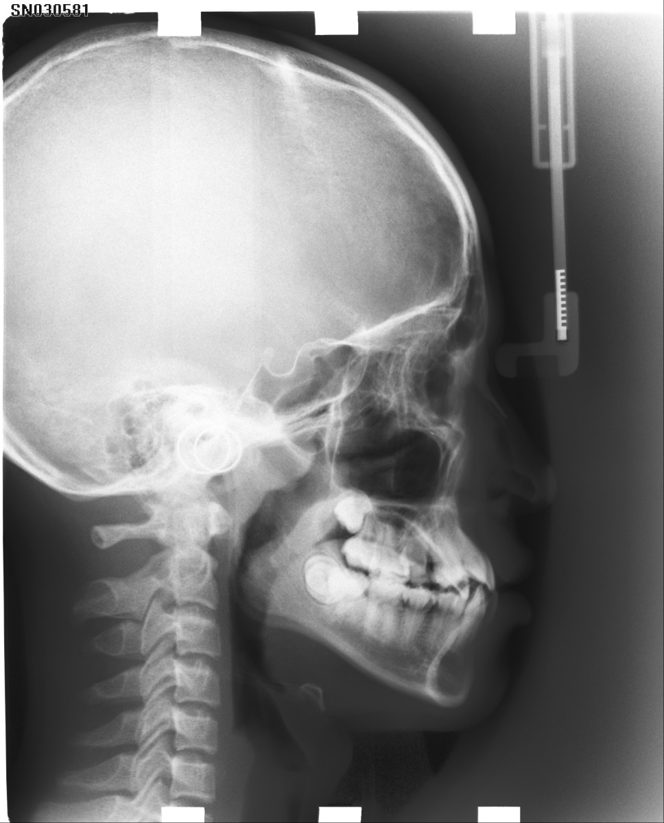
The proposed method is evaluated on two publicly available datasets for anatomical landmark localization. The first dataset consists of 895 radiographs of left hands of the Digital Hand Atlas Database System (Gertych et al., 2007; Zhang et al., 2009) with 37 annotated landmarks per image. Each image has been annotated by one of three experts. The second dataset consists of 400 lateral cephalograms with 19 annotated landmarks per image. This dataset has been used for the ISBI 2015 Cephalometric X-ray Image Analysis Challenge (Wang et al., 2016), in which each image has been annotated by both a senior and a junior radiologist.
Additional Annotations:
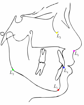
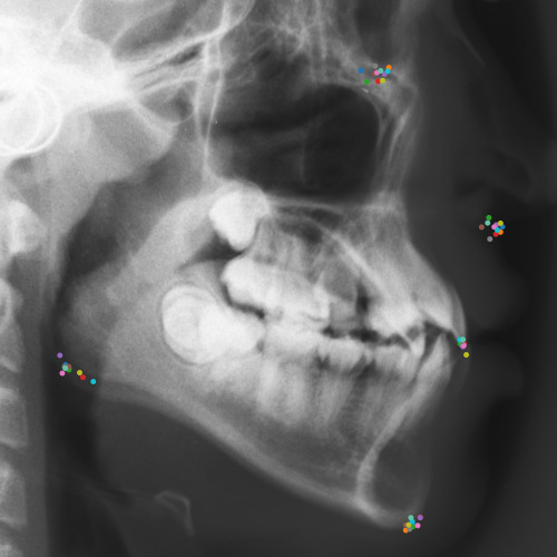
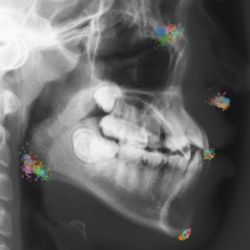
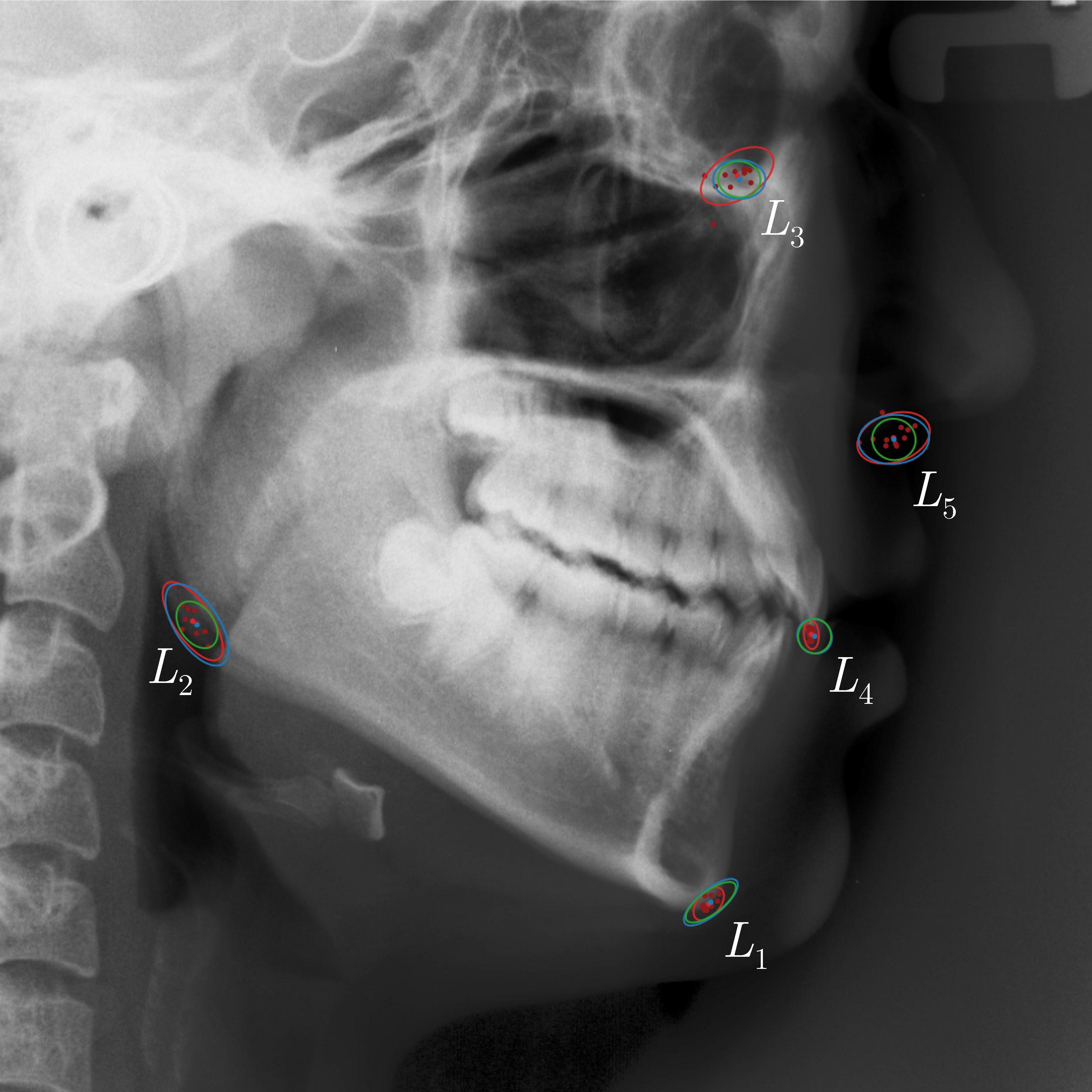
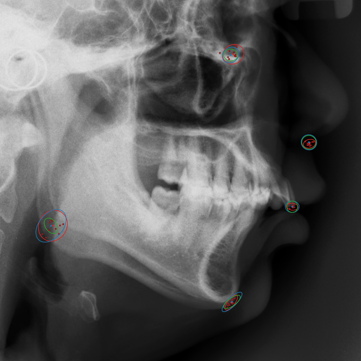
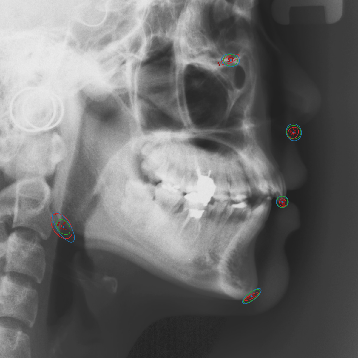
To assess the inter-observer variability and compare it with the predicted uncertainty, additional annotations for the dataset of cephalograms were obtained. 100 images were sampled randomly for which nine annotators experienced in medical image analysis labeled five representative landmarks of varying difficulty and ambiguity. The landmarks were chosen such that they cover a wide range of properties reflected by the shape and size of their expected distributions (see Fig. 2). Including the preexisting annotations of the senior and junior radiologist, this gives us a total of 11 annotations for the five selected landmarks111The code and additional annotations are available at:
https://github.com/christianpayer/MedicalDataAugmentationTool-HeatmapUncertainty. To estimate the distribution of the inter-observer variability, a Gaussian distribution was fitted to the 11 available annotations per landmark and image to retrieve the distribution parameters , and (see Eq. (4)). The inter-observer variability on the whole dataset for a landmark is calculated by taking the average over the distribution parameters for all images.
 |  |
 |  |
4.3 Metrics
For evaluating the landmark localization performance, the point-to-point error is used for the landmarks in image , which is defined as the Euclidean distance between the target coordinate and the predicted coordinate , i.e., . This allows calculation of sets of point-to-point errors, e.g., for all images of the dataset over all landmarks, over which the mean and standard deviation can be calculated. Additionally, we report the success detection rate, which is defined as the percentage of predicted landmarks that are within a certain point-to-point error radius for all images, i.e., .
While in most experiments only a single groundtruth coordinate per image and landmark is available, the groundtruth location in our inter-observer experiment is not only encoded as a single coordinate, but as a distribution. Such groundtruth distributions are compared to the distributions predicted by our method by analyzing the parameters of the Gaussian functions. As a measure of size of the distributions, we use the area encoded by the product of the extent of the major axis and minor axis, i.e., . As a measure of anisotropy, we use their ratio, i.e., . Additionally, to compare the predicted and groundtruth orientation for landmarks with a strong anisotropic distribution, the orientation angle with respect to the x-axis is reported.
5 Results and Discussion
In state-of-the-art methods for landmark localization using heatmap regression, only the maximum of the heatmap prediction is used to estimate the landmark location, while the remaining information in the heatmap is neglected. In this work, we show that the predicted heatmap additionally captures uncertainty information introduced by ambiguities when annotating the training dataset. Thus, we demonstrate that the parameters of the target heatmap Gaussian function estimated during training are modeling a dataset-based annotation uncertainty and the parameters of the Gaussian function fitted to the heatmap prediction models a sample-based annotation uncertainty during inference.
First, in Sec. 5.1 it is shown that our method, which takes the uncertainty of landmark localization into account, outperforms state-of-the-art methods in terms of both accuracy and robustness. In the following Sec. 5.2, we show that both dataset-based and sample-based annotation uncertainty correlate with the prediction error, while in Sec. 5.3, it is demonstrated that uncertainties also model the inter-observer variabilities. In Sec. 5.4, an ablation study is conducted to evaluate different strategies of using Gaussian functions in our method. In Sec. 5.5, we discuss how the inter-observer variability can influence the classification outcome of several clinical measures on lateral cephalograms.
5.1 Localization Accuracy and Robustness
| Method | PE (in mm) | in % | |||
|---|---|---|---|---|---|
| mean SD | mm | mm | mm | mm | |
| Lindner et al. (2015) | 0.85 1.01 | 93.68% | 96.32% | 97.69% | 98.95% |
| Urschler et al. (2018) | 0.80 0.93 | 92.19% | 94.85% | 96.57% | 98.46% |
| Payer et al. (2019) | 0.66 0.74 | 94.99% | 96.98% | 98.12% | 99.27% |
| -target,-fit | 0.61 0.67 | 95.93% | 97.80% | 98.72% | 99.54% |
| Method | PE (in mm) | in % | ||||
|---|---|---|---|---|---|---|
| mean SD | mm | mm | mm | mm | ||
| Test1 | Ibragimov et al. (2014) | 1.84 n/a | 71.72% | 77.40% | 81.93% | 88.04% |
| Lindner et al. (2015) | 1.67 n/a | 73.68% | 80.21% | 85.19% | 91.47% | |
| Zhong et al. (2019) | 1.12 0.88 | 86.91% | 91.82% | 94.88% | 97.90% | |
| Chen et al. (2019) | 1.17 n/a | 86.67% | 92.67% | 95.54% | 98.53% | |
| -target,-fit | 1.07 1.02 | 87.37% | 91.86% | 94.81% | 97.79% | |
| Test2 | Ibragimov et al. (2014) | 2.14 n/a | 62.74% | 70.47% | 76.53% | 85.11% |
| Lindner et al. (2015) | 1.92 n/a | 66.11% | 72.00% | 77.63% | 87.42% | |
| Zhong et al. (2019) | 1.42 0.84 | 76.00% | 82.90% | 88.74% | 94.32% | |
| Chen et al. (2019) | 1.48 n/a | 75.05% | 82.84% | 88.53% | 95.05% | |
| -target,-fit | 1.38 1.33 | 75.11% | 82.53% | 88.26% | 94.58% | |
| CV jun. | Lindner et al. (2015) | 1.20 n/a | 84.70% | 89.38% | 92.62% | 96.30% |
| Zhong et al. (2019) | 1.22 2.45 | 86.06% | 90.84% | 94.04% | 97.28% | |
| -target,-fit | 0.99 1.07 | 89.76% | 93.74% | 95.83% | 97.82% | |
In Tables 1 and 2, landmark prediction accuracy measured in point error (PE) and robustness measured in the success detection rate per radius () of our method is compared to the state-of-the-art on both the hand and cephalogram dataset, respectively. The reported values for the state-of-the-art methods are taken from the respective publications (Ibragimov et al., 2014; Lindner et al., 2015; Urschler et al., 2018; Payer et al., 2019; Zhong et al., 2019; Chen et al., 2019).
On a three-fold cross-validation (CV) of the dataset of left hand radiographs, our proposed method that uses an anisotropic Gaussian function to model both the target heatmap and the distribution of the heatmap prediction (-target,-fit) outperforms the previously published methods (Lindner et al., 2015; Urschler et al., 2018; Payer et al., 2019). Also, our method is compared to the winning methods of the ISBI Cephalometric X-ray Image Analysis Challenges in 2014 (Ibragimov et al., 2014) and 2015 (Lindner et al., 2015) as well as recent state-of-the-art methods on this dataset (Zhong et al., 2019; Chen et al., 2019). On both test sets Test1 and Test2, it can be observed that the methods using CNNs achieve similar results, while our method is the most accurate with the smallest PE. In terms of SDR, our method performs in-line with other methods, while Chen et al. (2019) perform slightly better in Test1 and Zhong et al. (2019) in Test2, respectively. Nevertheless, the results on Test1 and Test2 should be treated with caution because of the systematic shift of some landmarks (e.g. landmark 8 and 16) as compared to the annotations of the training data. The systematic shift has already been reported in (Lindner et al., 2016; Zhong et al., 2019) as well as in our MICCAI-UNSURE 2020 workshop paper (Payer et al., 2020). To mitigate the systematic shift, we follow previous work (Lindner et al., 2016; Zhong et al., 2019) and perform a four-fold cross-validation experiment trained and evaluated on the junior annotations only (CV jun.). Here, similar to the hand radiographs, it can be observed that our method that uses an anisotropic Gaussian function to model both the target heatmap and the distribution of the heatmap prediction (-target,-fit) leads to the best results, outperforming all other methods.
5.2 Correspondence of Heatmap Uncertainty and Localization Error
-target 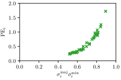 | 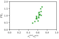 | 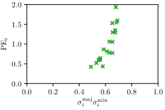 |
|---|---|---|
-fit 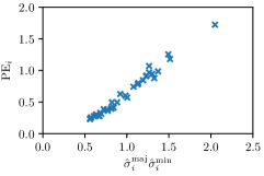 | 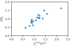 | 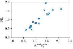 |
| hand | ceph. junior | ceph. mean |
| Input | -fit | -target | Offsets | -fit | -target |
|---|---|---|---|---|---|
 |  | ||||
 |  | ||||
 |  | ||||
 |  | ||||
| Input | -fit | -target | Offsets | -fit | -target |
|---|---|---|---|---|---|
 |  | ||||
 |  | ||||
 |  | ||||
 |  | ||||
In this work, we proposed to use parameters of the target Gaussian heatmaps to model a dataset-based annotation uncertainty (see Sec. 3.1) and parameters of a fitted Gaussian function to the predicted heatmaps to model a sample-based annotation uncertainty (see Sec. 3.2). In this section, it is shown that both sets of Gaussian parameters represent valid uncertainty measures by comparing the sizes of the Gaussians with the corresponding localization error for each landmark individually (see Fig. 3). For both the hand and cephalogram dataset, the size of the learned target Gaussians as well as the size of the fitted Gaussians are calculated as the product of the variances () averaged over the cross-validations or over all test images, respectively. It can be observed that both the target and fitted heatmap parameters correlate with the PE.
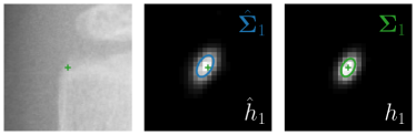
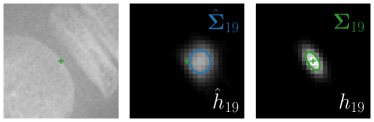
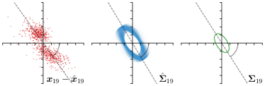
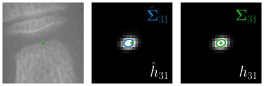
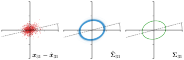
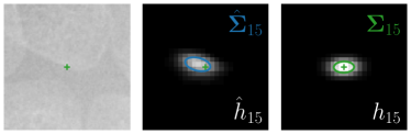
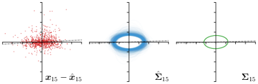
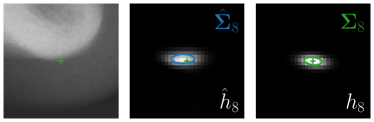
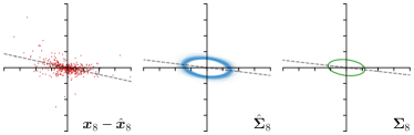
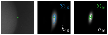
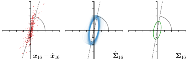
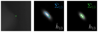
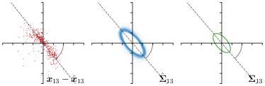
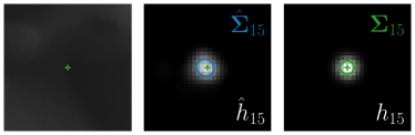
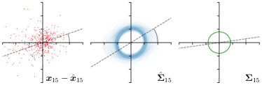
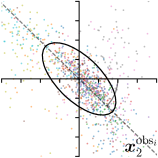
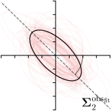
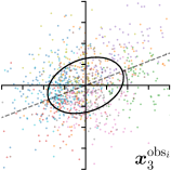
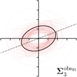
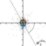
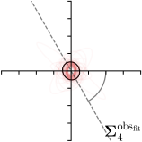
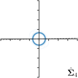
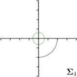
Our proposed method is also able to model directional uncertainties, which is visualized in Fig. 4 and 5 for selected landmarks. On the left side of the figures, the target and predicted heatmaps are superimposed with ellipses representing the target and fitted Gaussian parameters, respectively. Both target and predicted heatmaps are smaller for landmarks on distinct corners as compared to landmarks on edges. For landmarks on edges it can be observed that the heatmaps are oriented in direction of the underlying edges. Thus, for these landmarks the main sources for ambiguity are along the edges. In Fig. 4 and 5 (right) it is shown that both the learned target heatmap parameters and the fitted heatmap parameters correspond in orientation and size to the expected prediction-groundtruth offsets . For each landmark individually, the parameters of both target and predicted heatmaps are represented as ellipses centered at the origin, and plotted together for all images. To visualize the prediction-groundtruth offsets, individual predictions for all images are shown as points relative to their respective groundtruth positions, centered at the origin. From Fig. 4 and 5 it can be observed that the orientation and the size of both predicted and target heatmap parameters correspond to the prediction-groundtruth offsets. Overall, these results confirm that the target and the fitted parameters of the Gaussian functions are valid uncertainty measures.
5.3 Correspondence of Heatmap Uncertainty and Annotation Distribution
| Ann. | Ann.-fit | -fit | -target | |
|---|---|---|---|---|
 |  |  |  | |
 |  |  |  | |
 |  |  |  | |
 |  |  |  | |
 |  |  |  |
To reliably assess inter-observer variability, neither the hand dataset nor the cephalogram dataset can be used, as they were annotated by only one or two annotators per image, respectively. Therefore, we randomly chose 100 images of the cephalogram dataset and employed nine annotators experienced in medical image analysis to label five characteristic landmarks on each image. Combined with the junior and senior radiologist annotations already existing in the cephalogram dataset, this leads to a total of 11 annotations per image and landmark.
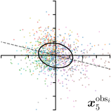
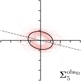
We trained a model of our proposed method (-target,-fit) on the mean coordinate according to the 11 annotations per image. The annotation and predicted distributions of the selected points are compared in Fig. 6. Similarly to how the prediction-groundtruth offsets are presented in Fig. 4, the annotation offsets for each annotator and image are visualized as points relative to the respective mean annotation of all 11 annotators, centered at the origin (Fig. 6, first column). To model the annotation distribution, a Gaussian distribution is fitted to the 11 annotations for each landmark and image individually. All annotation distributions as well as their mean are visualized as ellipses (Fig. 6, second column). The parameters of both predicted heatmaps (Fig. 6, third column) and target heatmaps (Fig. 6, last column) are represented as ellipses centered at the origin, plotted for all images. By visually comparing the size and the orientation of both predicted and target heatmap parameters with the annotation distributions, a correspondence can clearly be seen.
| Metric | Method | |||||
|---|---|---|---|---|---|---|
| Ratio | Ann. | 2.57 | 2.12 | 1.52 | 1.11 | 1.46 |
| -fit | 2.80 0.25 | 1.98 0.47 | 1.34 0.30 | 1.12 0.12 | 1.20 0.17 | |
| -target | 2.63 | 1.51 | 1.17 | 1.03 | 1.05 | |
| Product | Ann. | 0.37 | 2.73 | 2.34 | 0.26 | 1.13 |
| -fit | 0.63 0.07 | 1.40 0.35 | 0.86 0.18 | 0.44 0.08 | 0.98 0.24 | |
| -target | 0.48 | 0.62 | 0.52 | 0.40 | 0.62 | |
| Rotation (in degree) | Ann. | 39.33 | -44.30 | 20.97 | -60.34 | -13.98 |
| -fit | 37.48 2.72 | -56.62 14.82 | -0.88 35.90 | 1.25 57.68 | -30.52 36.00 | |
| -target | 36.79 | -54.39 | -7.10 | -89.47 | -14.04 |
When comparing the annotation offsets for different landmarks in Fig. 6, it can be observed that landmark 4 on the tip of the incisor has the best agreement among the annotators, due to its well defined location (see Fig. 2). Although landmark 5 also lies on an anatomically well defined location, due to low contrast in this region, its annotation variation is higher. Landmarks 2 and 3 were the most problematic ones to annotate. Landmark 2 is challenging, because its position has to be estimated by the annotators in between the left and right mandible, when they are not aligned and therefore, are not seen as a single edge in the lateral cephalograms. Landmark 3 lies on an edge of a bone within the skull that is challenging to recognize and becomes ambiguous if the head is tilted. For landmark 1 that lies on the tip of the chin, it can be seen that the annotators correctly identified the edge of the chin, however, identifying the exact position along the edge of the chin was challenging. Thus, the annotation distribution for this landmark has a clear dominant direction.
In all the previous works based on heatmap regression, the target heatmaps are modeled as isotropic functions. However, from the annotation distributions in Fig. 6, second column, clear anisotropic orientations of the inter-observer variabilities of the landmarks located at smooth edges, i.e., landmark 1 and 2 are observable. Thus, to estimate the inter-observer variability, in this work, we used anisotropic Gaussian functions for target heatmaps, as well as to model the predicted distribution. This enables our method to successfully model the inter-observer variability as can be seen when comparing both the predicted Gaussian functions in the third and the learned target Gaussian functions in the last column to the annotation distributions in the second column of Fig. 6.
To quantitatively validate this correspondence between the parameters of the Gaussian functions of our proposed method and the annotation distribution, we present the ratio and product of the extent of the major axis and minor axis as well as the orientation angle of the Gaussian functions in Table 3. The product of the extents of the major axis and minor axis shows that the parameters of both target and average fitted Gaussians have the tendencies of underestimating the size of the annotation uncertainty for landmarks with a larger inter-observer variability (landmark 2, 3, 5). Nevertheless, for the landmarks with lower inter-observer variability (landmark 1, 4), the size of the Gaussian functions is in range with the size of the annotation uncertainty. From the ratio of the extent of the major axis and minor axis , it can be observed that our method is not only able to model isotropic annotation distributions (landmark 3, 4, 5) but also anisotropic ones (landmark 1, 2). It is interesting to see that both ratios of the target and the average fitted Gaussian parameters are similar to the ratio of the annotation distributions. Furthermore, the rotation angles of the Gaussian functions also approximate the rotation angle of the annotation distribution for the anisotropic landmarks well.
 |  |  |
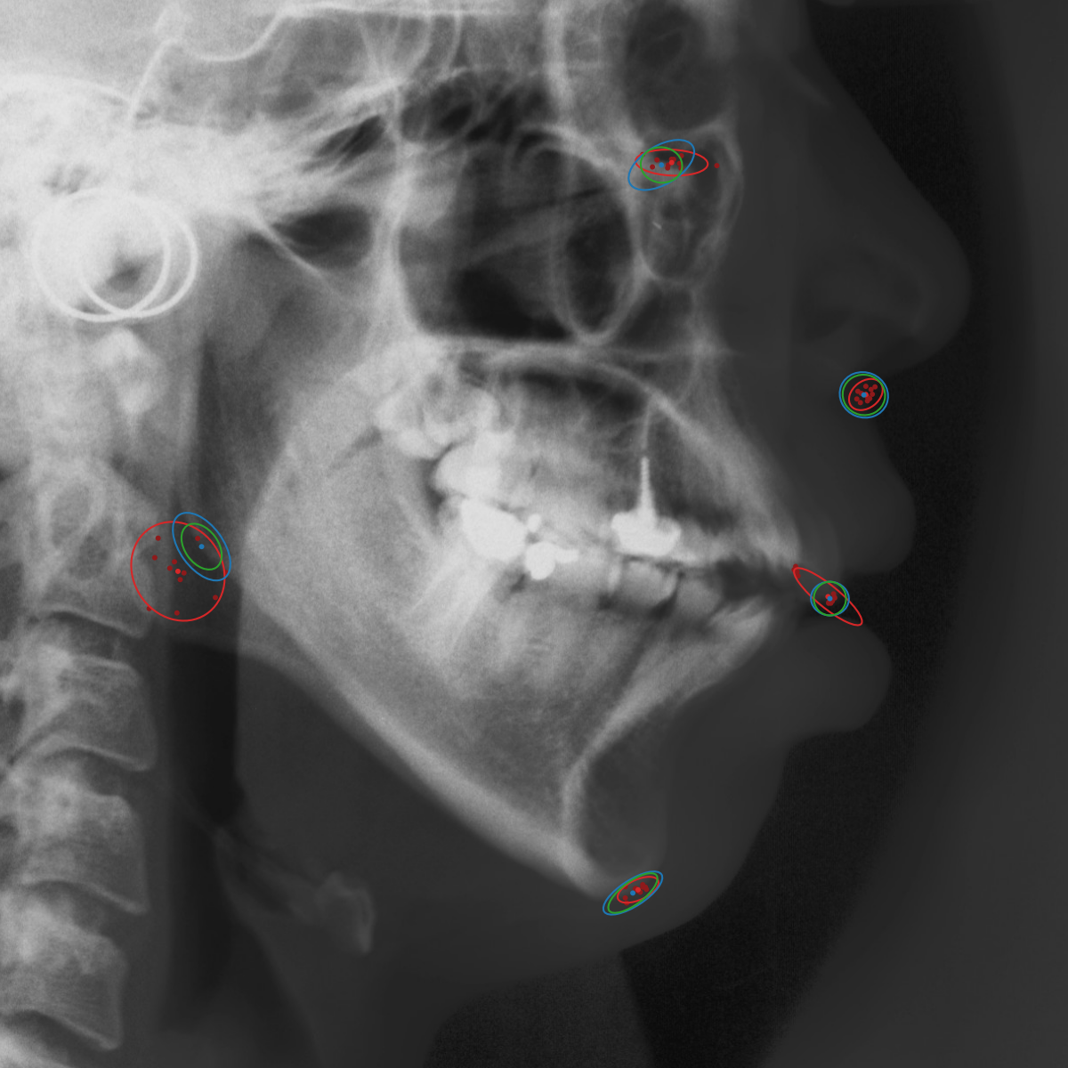 | 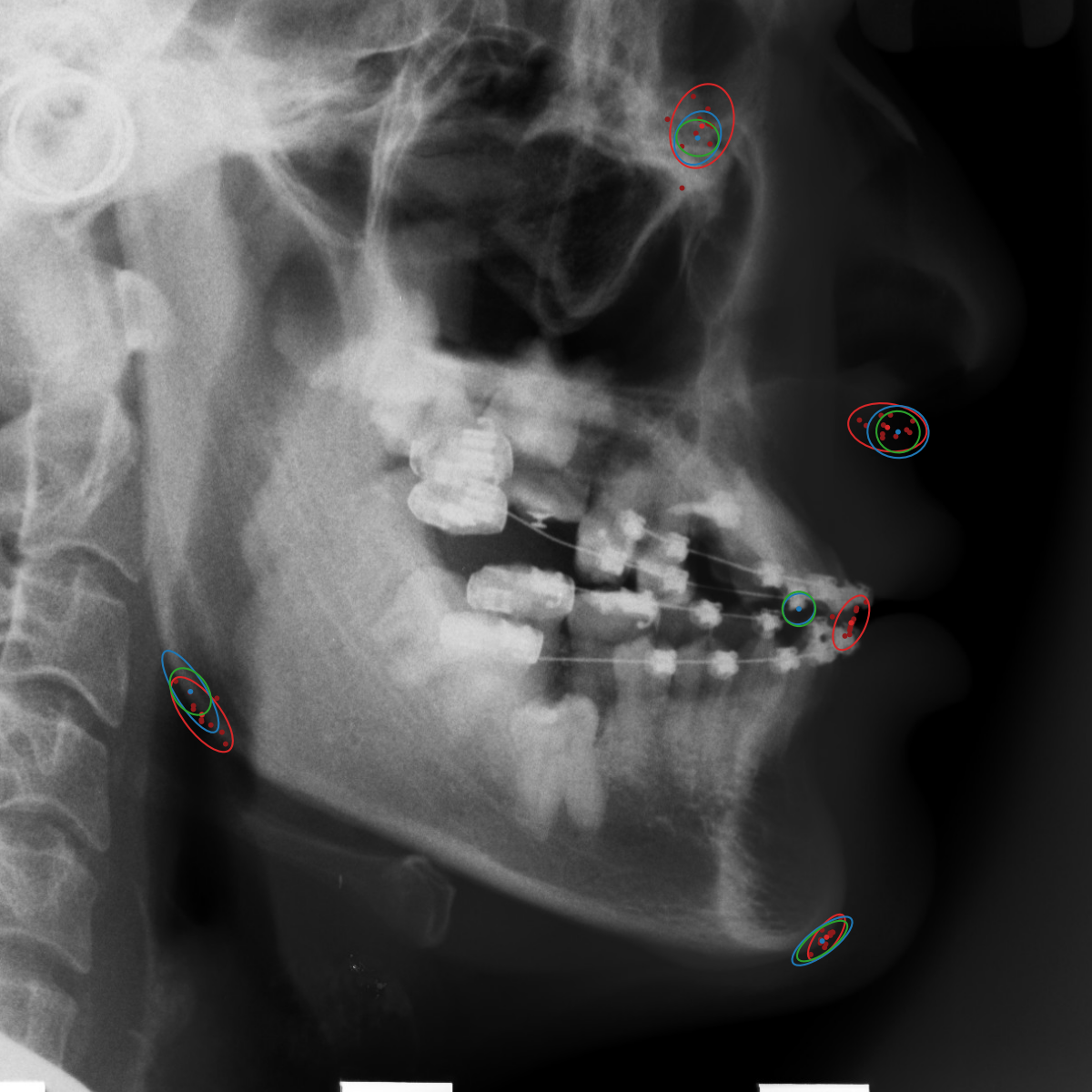 | 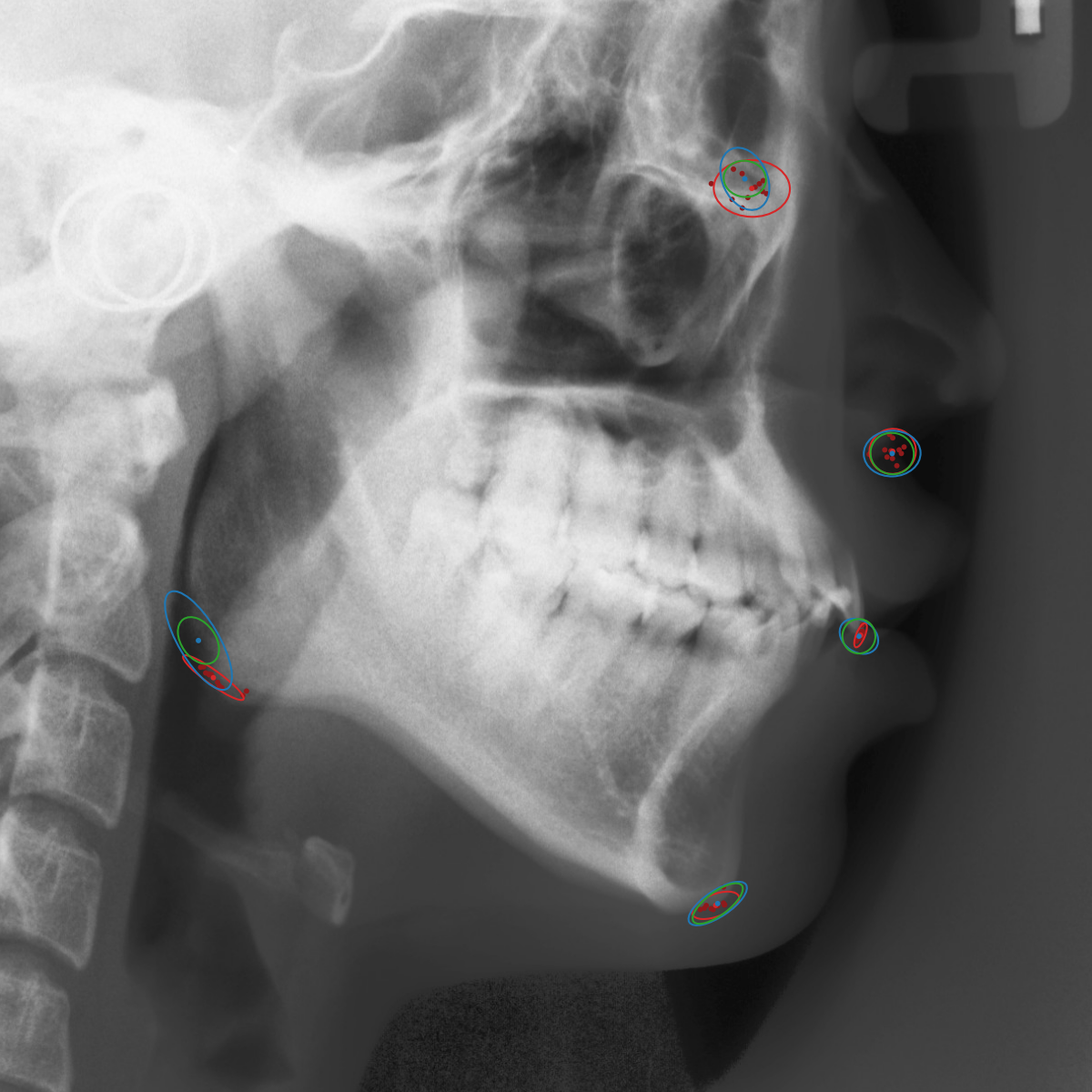 |
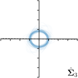
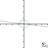
Qualitative results of the landmark predictions as well as the predicted distributions for each landmark are presented in Fig. 7 for selected images. The visualized points are the 11 inter-observer annotations (dark red), their mean position (red) and the landmark predictions of our model (blue). The red ellipses represent the distributions fitted to the 11 annotations. The sample-based uncertainties and the dataset-based uncertainties are represented as blue and green ellipses, respectively. For the depicted images, it can be seen that most landmark predictions closely match to the mean of the 11 annotations, while the predicted uncertainties are similar to the annotation distributions. Discrepancy between the inter-observer annotations and uncertainties predicted by our method were primarily caused by landmarks that where difficult to recognize in a given image (landmark 2, bottom left and landmark 4, bottom middle) or by landmarks with high ambiguity (e.g., landmark 3, bottom middle and landmark 2 bottom right). Nevertheless, the predicted sample-based uncertainties are similar to the annotation distributions even when the dataset-based uncertainty of a landmark is too restrictive as, e.g., for landmark 2 (top middle), where both mandibles are visible due to the head being tilted.
5.4 Ablation Study
| Method | Metric | |||||
| Ann. | 2.57 | 2.12 | 1.52 | 1.11 | 1.46 | |
| 0.37 | 2.73 | 2.34 | 0.26 | 1.13 | ||
| (in degree) | 39.33 | -44.30 | 20.97 | -60.34 | -13.98 | |
| -fit | 2.80 0.25 | 1.98 0.47 | 1.34 0.30 | 1.12 0.12 | 1.20 0.17 | |
| 0.63 0.07 | 1.40 0.35 | 0.86 0.18 | 0.44 0.08 | 0.98 0.24 | ||
| (in degree) | 37.48 2.72 | -56.62 14.82 | -0.88 35.90 | 1.25 57.68 | -30.52 36.00 | |
| -tar., | 2.63 | 1.51 | 1.17 | 1.03 | 1.05 | |
| 0.48 | 0.62 | 0.52 | 0.40 | 0.62 | ||
| (in degree) | 36.79 | -54.39 | -7.10 | -89.47 | -14.04 | |
| PE (in mm) | 0.34 0.25 | 1.31 0.94 | 0.94 0.67 | 0.41 0.76 | 0.65 0.47 | |
| -fit | 1.35 0.14 | 1.70 0.44 | 1.28 0.22 | 1.13 0.16 | 1.21 0.19 | |
| 0.76 0.07 | 1.51 0.38 | 0.88 0.19 | 0.45 0.11 | 1.02 0.28 | ||
| (in degree) | 37.16 9.07 | -56.89 25.12 | 2.71 55.33 | 31.51 54.57 | -40.34 44.71 | |
| -tar., | 1.00 | 1.00 | 1.00 | 1.00 | 1.00 | |
| 0.52 | 0.63 | 0.52 | 0.39 | 0.62 | ||
| (in degree) | - | - | - | - | - | |
| PE (in mm) | 0.35 0.28 | 1.38 0.99 | 1.00 0.72 | 0.40 0.75 | 0.65 0.45 | |
| -fit | 1.29 0.13 | 1.68 0.39 | 1.27 0.24 | 1.10 0.09 | 1.17 0.14 | |
| 0.90 0.09 | 1.46 0.46 | 0.96 0.20 | 0.70 0.10 | 0.98 0.22 | ||
| (in degree) | 36.73 11.78 | -56.92 22.70 | -2.04 55.45 | 25.23 49.33 | -34.09 53.11 | |
| =3, | 1.00 | 1.00 | 1.00 | 1.00 | 1.00 | |
| 0.66 | 0.66 | 0.66 | 0.66 | 0.66 | ||
| (in degree) | - | - | - | - | - | |
| PE (in mm) | 0.35 0.24 | 1.29 0.92 | 0.97 0.69 | 0.42 0.77 | 0.64 0.51 | |
| MCD-max | 2.61 0.86 | 4.84 3.36 | 2.31 1.55 | 1.73 0.97 | 1.96 1.11 | |
| 0.01 0.00 | 0.27 0.55 | 0.06 0.09 | 0.02 0.11 | 0.02 0.04 | ||
| (in degree) | 33.89 14.57 | -58.03 28.26 | 19.70 50.21 | 51.33 32.61 | 32.36 44.69 | |
| PE (in mm) | 0.35 0.25 | 1.31 0.87 | 0.99 0.69 | 0.39 0.66 | 0.65 0.46 | |
| MCD--fit | 1.31 0.13 | 1.78 0.47 | 1.27 0.23 | 1.10 0.10 | 1.17 0.13 | |
| 0.89 0.08 | 1.48 0.40 | 1.01 0.22 | 0.72 0.13 | 1.01 0.22 | ||
| (in degree) | 36.96 9.61 | -56.74 19.44 | 4.26 59.02 | 25.17 49.42 | -29.44 48.50 | |
| PE (in mm) | 0.34 0.24 | 1.34 1.04 | 0.97 0.68 | 0.42 0.77 | 0.65 0.50 |
Ann. | 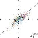 | 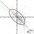 | ||
-tar.,-fit | 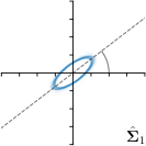 | 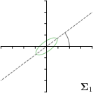 | 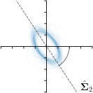 | 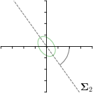 |
-tar.,-fit | 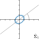 | 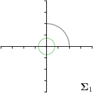 | 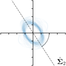 | 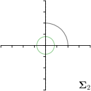 |
=3,-fit | 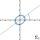 | 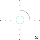 | 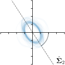 |  |
MCD-,max | 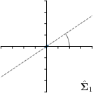 |  | 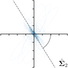 |  |
MCD-,-fit | 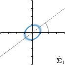 |  | 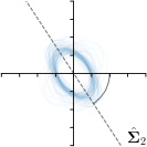 |  |
Different strategies of using the Gaussian function to model both the target heatmap and the distribution of the heatmap prediction are investigated. We distinguish methods based on whether the target heatmap used during training is defined as a Gaussian function with a fixed isotropic variance (=3), learned isotropic variance (-target) or learned anisotropic covariance (-target). For the fixed isotropic variance, the value was chosen, as it showed to have a good trade-off between PE and . As already defined, our main method uses the Gaussian function with anisotropic covariance during both training and inference, which we named -target,-fit. For comparison with state-of-the-art methods estimating uncertainty, we implemented two approaches using MCD as described in Sec. 4. The cephalogram dataset with our additional annotations was used for method comparison as well as the same visualizations and measures as in the previous Sec. 5.3. Results of these comparisons for two selected landmarks with the highest anisotropy are shown in Fig. 8, while the quantitative results for all five landmarks are shown in Table 4.
When comparing the localization accuracy in terms of PE, all different heatmap target and fitting strategies perform similarly well as can be seen in Table 4. Similarly as in Sec. 5.3, it can be seen that both target and predicted heatmaps have the tendency of underestimating the annotation distribution size for landmarks having a large inter-observer variability. When looking at the distributions modeled by the target heatmaps in Fig. 8, it can be observed that strategies using either fixed () or learned isotropic values (-target) have no capacity of modeling the annotation distribution. Interestingly, when fitting anisotropic Gaussian functions to the heatmaps predicted by both of these strategies, the orientation angles of the inter-observer variability are successfully estimated. However, the ratio of in Table 4 shows that our final model, which uses anisotropic Gaussian functions for both target heatmaps and prediction fitting (-target,-fit), better captures the anisotropy of the annotator distributions.
Our method is also compared with the state-of-the-art method MCD for estimating uncertainties adapted to the landmark localization task, where the uncertainty is either computed as the variance of a set of stochastic forward predictions (MCD-,max) or estimated by fitting a Gaussian to an accumulated set of stochastic heatmaps (MCD-,-fit). Since fixed target heatmaps were used to be consistent with related work, only the variances respectively the parameters of the fitted Gaussians are compared with the annotation distributions. As can be seen in Table 4, there is no significant difference when comparing MCD to any of our strategies in terms of the PE. However, MCD-,max is not capable of estimating the size of the annotation distributions , due to the predicted coordinates being very similar for all passes which leads to an underestimation. Moreover, the ratio of is also unreliable for this method. The method MCD-,-fit has a similar performance as our strategy -target,-fit, which was to be expected as the uncertainty is also estimated by fitting a Gaussian.
5.5 Prediction Uncertainty in Clinical Measurements
| Classification Accuracy |
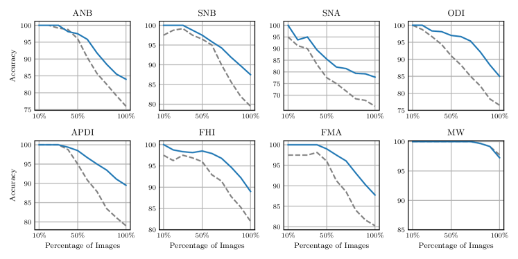 |
In clinical practice utilizing computer aided diagnosis, often only the most probable landmark prediction is used, while the uncertainty distribution of the prediction is ignored leading to overconfidence in calculated clinical measurements. To show the importance of considering the annotation uncertainty of the dataset used for training the machine learning model, we evaluate the influence of the predicted landmark localization uncertainty to the classification accuracy of clinical measurements for orthodontic analysis and treatment planning. For this experiment, the same eight measurements that classify anatomical abnormalities as described in Wang et al. (2016) and listed in Fig. 9 are used.
To show the correlation of the predicted landmark localization uncertainty with the classification accuracy, we first calculated how the classification prediction is affected by the predicted landmark distributions. Thus, for each patient and measurement, 10,000 points are sampled from each landmark distribution predicted by our -target,-fit method trained using the junior annotations to calculate 10,000 classification outcomes in the four-fold cross-validation setup (CV jun.) that we used before in Sec. 5.1. For each patient and measurement, the entropy of the class probabilities is used to obtain the classification uncertainty, while the classification accuracy is calculated as the agreement of the most probable class prediction with the junior annotation.
To verify that such a calculated entropy is a valid measure of uncertainty, we compare the classification uncertainty with the classification accuracy, for each clinical measurement independently. Fig. 9 visualizes the average accuracy that is calculated by increasing the number of considered patients, ordered from lower to higher uncertainty. For all clinical measurements, the blue line in Fig. 9 shows that the average classification accuracy is decreasing when the number of images with higher classification uncertainty is increasing. Thus, our experiment shows that the predicted landmark localization uncertainty can also be used to model classification uncertainty influencing the classification accuracy.
Additionally, the dashed line in Fig. 9 shows the classification accuracy of the senior as compared to the junior annotator, for the same order of images as used to generate the blue line. When comparing the dashed with the blue line, it can be seen that the classification agreement of the senior to the junior is in general lower as compared to our method, which can be explained by our model being trained on the junior annotation. However, it is more interesting to see that by ordering the images according to the uncertainty of our model, the accuracy of the senior’s classification compared to the junior’s is also decreasing. An interesting extension would be to estimate the optimal heatmap size directly by maximizing the classification accuracy, however, this would go beyond the scope of this work focusing on landmark localization. Nevertheless, the experiment in this subsection further confirms that our method was able to identify samples with higher ambiguities in annotation.
6 Conclusion
In the state-of-the-art methods for landmark localization, only the most probable prediction is used to estimate the landmark location, without considering the location distribution. In this work, it was shown that the heatmap prediction can be used to model the location distribution reflecting the aleatoric uncertainty coming from ambiguous annotations. By learning anisotropic Gaussian parameters of the target heatmaps during optimization, our method is able to model annotation ambiguities of the entire training dataset. Furthermore, by fitting anisotropic Gaussian functions to the predicted heatmaps during inference, our method is also able to model the prediction uncertainty of individual samples. Additionally to the state-of-the-art results on both evaluated datasets, i.e., radiographs of left hands and lateral cephalograms, the results show that the size of the Gaussian function modeling the target heatmap as well as the size of the Gaussian function fitted to the predicted heatmap correlate with the localization accuracy. Finally, the experiment on the cephalogram dataset annotated by 11 observers has shown that our method successfully models the inter-observer variability. By measuring how the classification of anatomical abnormalities in lateral cephalograms is influenced by the predicted location uncertainty, we have shown the importance of integrating the uncertainty into decision making to identify overconfident predictions, thus, potentially improving patient treatment.
Acknowledgments
This work was supported by the Austrian Research Promotion Agency (FFG): 871262.
Ethical Standards
The work follows appropriate ethical standards in conducting research and writing the manuscript, following all applicable laws and regulations regarding treatment of animals or human subjects.
Conflicts of Interest
We declare we don’t have conflicts of interest.
References
- Ayhan and Berens (2018) Murat Seçkin Ayhan and Philipp Berens. Test-time Data Augmentation for Estimation of Heteroscedastic Aleatoric Uncertainty in Deep Neural Networks. Medical Imaging with Deep Learning, 2018.
- Beichel et al. (2005) Reinhard Beichel, Horst Bischof, Franz Leberl, and Milan Sonka. Robust Active Appearance Models and Their Application to Medical Image Analysis. IEEE Transactions on Medical Imaging, 24(9):1151–1169, 2005. ISSN 0278-0062.
- Bier et al. (2018) Bastian Bier, Mathias Unberath, Jan-Nico Zaech, Javad Fotouhi, Mehran Armand, Greg Osgood, Nassir Navab, and Andreas Maier. X-ray-transform Invariant Anatomical Landmark Detection for Pelvic Trauma Surgery. In Proceedings of the International Conference on Medical Image Computing and Computer-Assisted Intervention, pages 55–63, 2018. ISBN 9783030009366.
- Bier et al. (2019) Bastian Bier, Florian Goldmann, Jan-Nico Zaech, Javad Fotouhi, Rachel Hegeman, Robert Grupp, Mehran Armand, Greg Osgood, Nassir Navab, Andreas Maier, and Mathias Unberath. Learning to Detect Anatomical Landmarks of the Pelvis in X-Rays from Arbitrary Views. International Journal of Computer Assisted Radiology and Surgery, 14(9):1463–1473, 2019. ISSN 1861-6410.
- Blundell et al. (2015) Charles Blundell, Julien Cornebise, Koray Kavukcuoglu, and Daan Wierstra. Weight Uncertainty in Neural Networks. In International Conference on Machine Learning, 2015. ISBN 9781510810587.
- Branch et al. (1999) Mary Ann Branch, Thomas F. Coleman, and Yuying Li. A Subspace, Interior, and Conjugate Gradient Method for Large-Scale Bound-Constrained Minimization Problems. SIAM Journal on Scientific Computing, 21(1):1–23, 1999. ISSN 1064-8275.
- Camarasa et al. (2020) Robin Camarasa, Daniel Bos, Jeroen Hendrikse, Paul Nederkoorn, Eline Kooi, Aad van der Lugt, and Marleen de Bruijne. Quantitative Comparison of Monte-Carlo Dropout Uncertainty Measures for Multi-class Segmentation. In Uncertainty for Safe Utilization of Machine Learning in Medical Imaging, and Graphs in Biomedical Image Analysis, pages 32–41. Springer, 2020.
- Chen et al. (2019) L. Chen, H. Su, and Q. Ji. Face Alignment With Kernel Density Deep Neural Network. In Proceedings of IEEE International Conference on Computer Vision, pages 6991–7001, 2019. doi: 10.1109/ICCV.2019.00709.
- Chen et al. (2019) Runnan Chen, Yuexin Ma, Nenglun Chen, Daniel Lee, and Wenping Wang. Cephalometric Landmark Detection by Attentive Feature Pyramid Fusion and Regression-Voting. In Proceedings of the International Conference on Medical Image Computing and Computer-Assisted Intervention, pages 873–881, 2019. ISBN 9783030322472.
- Chotzoglou and Kainz (2019) Elisa Chotzoglou and Bernhard Kainz. Exploring the Relationship Between Segmentation Uncertainty, Segmentation Performance and Inter-observer Variability with Probabilistic Networks. In Large-Scale Annotation of Biomedical Data and Expert Label Synthesis and Hardware Aware Learning for Medical Imaging and Computer Assisted Intervention, pages 51–60. Springer, 2019.
- Gal and Ghahramani (2016) Yarin Gal and Zoubin Ghahramani. Dropout as a Bayesian Approximation: Representing Model Uncertainty in Deep Learning. In Proceedings of the International Conference on Machine Learning, pages 1050–1059, 2016. ISBN 9781510829008.
- Gertych et al. (2007) Arkadiusz Gertych, Aifeng Zhang, James Sayre, Sylwia Pospiech-Kurkowska, and H.K. Huang. Bone Age Assessment of Children Using a Digital Hand Atlas. Computerized Medical Imaging and Graphics, 31(4-5):322–331, 2007. ISSN 08956111.
- Gundavarapu et al. (2019) Nitesh B. Gundavarapu, Divyansh Srivastava, Rahul Mitra, Abhishek Sharma, and Arjun Jain. Structured Aleatoric Uncertainty in Human Pose Estimation. In Proceedings of the IEEE Computer Society Conference on Computer Vision and Pattern Recognition, June 2019.
- Gunning et al. (2019) David Gunning, Mark Stefik, Jaesik Choi, Timothy Miller, Simone Stumpf, and Guang-Zhong Yang. XAI - Explainable Artificial Intelligence. Science Robotics, 4(37):eaay7120, 2019. ISSN 2470-9476.
- Heimann and Meinzer (2009) Tobias Heimann and Hans Peter Meinzer. Statistical Shape Models for 3D Medical Image Segmentation: A Review. Medical Image Analysis, 13(4):543–563, 2009. ISSN 13618415.
- Ibragimov et al. (2014) Bulat Ibragimov, Boštjan Likar, Franjo Pernuš, and Tomaž Vrtovec. Shape Representation for Efficient Landmark-Based Segmentation in 3-D. IEEE Transactions on Medical Imaging, 33(4):861–874, 2014. ISSN 02780062.
- Johnson and Christensen (2002) Hans J. Johnson and Gary E. Christensen. Consistent Landmark and Intensity-Based Image Registration. IEEE Transactions on Medical Imaging, 21(5):450–461, 2002. ISSN 02780062.
- Jungo et al. (2018) Alain Jungo, Raphael Meier, Ekin Ermis, Marcela Blatti-Moreno, Evelyn Herrmann, Roland Wiest, and Mauricio Reyes. On the Effect of Inter-observer Variability for a Reliable Estimation of Uncertainty of Medical Image Segmentation. In Proceedings of the International Conference on Medical Image Computing and Computer-Assisted Intervention, pages 682–690. Springer, 2018.
- Kendall and Gal (2017) Alex Kendall and Yarin Gal. What Uncertainties Do We Need in Bayesian Deep Learning for Computer Vision? In Advances in Neural Information Processing Systems, pages 5574–5584, 2017.
- Kwon et al. (2020) Yongchan Kwon, Joong Ho Won, Beom Joon Kim, and Myunghee Cho Paik. Uncertainty Quantification using Bayesian Neural Networks in Classification: Application to Biomedical Image Segmentation. Computational Statistics and Data Analysis, 2020. ISSN 01679473. doi: 10.1016/j.csda.2019.106816.
- Leibig et al. (2017) Christian Leibig, Vaneeda Allken, Murat Seçkin Ayhan, Philipp Berens, and Siegfried Wahl. Leveraging Uncertainty Information from Deep Neural Networks for Disease Detection. Scientific Reports, 7(1):1–14, 2017.
- Lindner et al. (2015) Claudia Lindner, Paul A. Bromiley, Mircea C. Ionita, and Tim F. Cootes. Robust and Accurate Shape Model Matching Using Random Forest Regression-Voting. IEEE Transactions on Pattern Analysis and Machine Intelligence, 37(9):1862–1874, 2015. ISSN 0162-8828.
- Lindner et al. (2016) Claudia Lindner, Ching-Wei Wang, Cheng-Ta Huang, Chung-Hsing Li, Sheng-Wei Chang, and Tim F. Cootes. Fully Automatic System for Accurate Localisation and Analysis of Cephalometric Landmarks in Lateral Cephalograms. Scientific Reports, 6:33581, 2016.
- Liu et al. (2019) Zhiwei Liu, Xiangyu Zhu, Guosheng Hu, Haiyun Guo, Ming Tang, Zhen Lei, Neil M. Robertson, and Jinqiao Wang. Semantic Alignment: Finding Semantically Consistent Ground-Truth for Facial Landmark Detection. In Proceedings of the IEEE Conference on Computer Vision and Pattern Recognition, pages 3462–3471. IEEE, jun 2019. ISBN 978-1-7281-3293-8. doi: 10.1109/CVPR.2019.00358. URL https://ieeexplore.ieee.org/document/8953973/.
- Mader et al. (2019) Alexander Oliver Mader, Cristian Lorenz, Jens von Berg, and Carsten Meyer. Automatically Localizing a Large Set of Spatially Correlated Key Points: A Case Study in Spine Imaging. In Proceedings of the International Conference on Medical Image Computing and Computer-Assisted Intervention, pages 384–392, 2019. ISBN 978-3-030-32226-7.
- Mobiny et al. (2019) Aryan Mobiny, Aditi Singh, and Hien Van Nguyen. Risk-Aware Machine Learning Classifier for Skin Lesion Diagnosis. Journal of Clinical Medicine, 2019. ISSN 2077-0383. doi: 10.3390/jcm8081241.
- Nair et al. (2020) Tanya Nair, Doina Precup, Douglas L. Arnold, and Tal Arbel. Exploring Uncertainty Measures in Deep Networks for Multiple Sclerosis Lesion Detection and Segmentation. Medical Image Analysis, 2020. ISSN 13618423.
- Newell et al. (2016) Alejandro Newell, Kaiyu Yang, and Jia Deng. Stacked Hourglass Networks for Human Pose Estimation. In Proceedings of the European Conference on Computer Vision, pages 483–499, 2016. ISBN 9783319464848.
- Payer et al. (2016) Christian Payer, Darko Štern, Horst Bischof, and Martin Urschler. Regressing Heatmaps for Multiple Landmark Localization Using CNNs. In Proceedings of the International Conference on Medical Image Computing and Computer-Assisted Intervention, pages 230–238, 2016. ISBN 9783319467221.
- Payer et al. (2019) Christian Payer, Darko Štern, Horst Bischof, and Martin Urschler. Integrating Spatial Configuration into Heatmap Regression Based CNNs for Landmark Localization. Medical Image Analysis, 54:207–219, 2019. ISSN 13618415.
- Payer et al. (2020) Christian Payer, Martin Urschler, Horst Bischof, and Darko Štern. Uncertainty Estimation in Landmark Localization Based on Gaussian Heatmaps. In Uncertainty for Safe Utilization of Machine Learning in Medical Imaging, and Graphs in Biomedical Image Analysis, pages 42–51. Springer, 2020.
- Roy et al. (2018) Abhijit Guha Roy, Sailesh Conjeti, Nassir Navab, and Christian Wachinger. Inherent Brain Segmentation Quality Control from Fully ConvNet Monte Carlo Sampling. In Proceedings of the International Conference on Medical Image Computing and Computer-Assisted Intervention, pages 664–672. Springer, 2018.
- Sedghi et al. (2019) Alireza Sedghi, Tina Kapur, Jie Luo, Parvin Mousavi, and William M Wells. Probabilistic Image Registration via Deep Multi-class Classification: Characterizing Uncertainty. In Uncertainty for Safe Utilization of Machine Learning in Medical Imaging and Clinical Image-Based Procedures, pages 12–22. Springer, 2019.
- Shridhar et al. (2019) Kumar Shridhar, Felix Laumann, and Marcus Liwicki. A Comprehensive Guide to Bayesian Convolutional Neural Network with Variational Inference. arXiv preprint arXiv:1901.02731, 2019.
- Srivastava et al. (2014) Nitish Srivastava, Geoffrey Hinton, Alex Krizhevsky, Ilya Sutskever, and Ruslan Salakhutdinov. Dropout: A Simple Way to Prevent Neural Networks from Overfitting. Journal of Machine Learning Research, 15(1):1929–1958, 2014. ISSN 15337928.
- Štern et al. (2011) Darko Štern, Boštjan Likar, Franjo Pernuš, and Tomaž Vrtovec. Parametric Modelling and Segmentation of Vertebral Bodies in 3D CT and MR Spine Images. Physics in Medicine and Biology, 56(23):7505–7522, 2011. ISSN 00319155.
- Štern et al. (2019) Darko Štern, Christian Payer, and Martin Urschler. Automated Age Estimation from MRI Volumes of the Hand. Medical Image Analysis, 58:101538, 2019. ISSN 13618415.
- Tompson et al. (2014) Jonathan Tompson, Arjun Jain, Yann LeCun, and Christoph Bregler. Joint Training of a Convolutional Network and a Graphical Model for Human Pose Estimation. In Advances in Neural Information Processing Systems, pages 1799–1807, 2014.
- Toshev and Szegedy (2014) Alexander Toshev and Christian Szegedy. DeepPose: Human Pose Estimation via Deep Neural Networks. In Proceedings of the IEEE Conference on Computer Vision and Pattern Recognition, pages 1653–1660, 2014. ISBN 978-1-4799-5118-5.
- Urschler et al. (2006) Martin Urschler, Christopher Zach, Hendrik Ditt, and Horst Bischof. Automatic Point Landmark Matching for Regularizing Nonlinear Intensity Registration: Application to Thoracic CT Images. In Proceedings of the International Conference on Medical Image Computing and Computer-Assisted Intervention, pages 710–717, 2006. ISBN 3-540-44727-X.
- Urschler et al. (2018) Martin Urschler, Thomas Ebner, and Darko Štern. Integrating Geometric Configuration and Appearance Information into a Unified Framework for Anatomical Landmark Localization. Medical Image Analysis, 43:23–36, 2018. ISSN 13618415.
- Vrtovec et al. (2009) Tomaž Vrtovec, Franjo Pernuš, and Boštjan Likar. A Review of Methods for Quantitative Evaluation of Spinal Curvature. European Spine Journal, 18(5):593–607, 2009. ISSN 0940-6719.
- Wang et al. (2016) Ching Wei Wang, Cheng Ta Huang, Jia Hong Lee, Chung Hsing Li, Sheng Wei Chang, Ming Jhih Siao, Tat Ming Lai, Bulat Ibragimov, Tomaž Vrtovec, Olaf Ronneberger, Philipp Fischer, Tim F. Cootes, and Claudia Lindner. A Benchmark for Comparison of Dental Radiography Analysis Algorithms. Medical Image Analysis, 31:63–76, 2016. ISSN 13618423.
- Wang et al. (2019a) Guotai Wang, Wenqi Li, Michael Aertsen, Jan Deprest, Sébastien Ourselin, and Tom Vercauteren. Aleatoric Uncertainty Estimation with Test-time Augmentation for Medical Image Segmentation with Convolutional Neural Networks. Neurocomputing, 338:34–45, 2019a.
- Wang et al. (2019b) Guotai Wang, Wenqi Li, Sébastien Ourselin, and Tom Vercauteren. Automatic Brain Tumor Segmentation Based on Cascaded Convolutional Neural Networks With Uncertainty Estimation. Frontiers in Computational Neuroscience, 13, 2019b. ISSN 1662-5188.
- Wei et al. (2016) Shih-En Wei, Varun Ramakrishna, Takeo Kanade, and Yaser Sheikh. Convolutional Pose Machines. In Proceedings of the IEEE Conference on Computer Vision and Pattern Recognition, pages 4724–4732, 2016. ISBN 978-1-4673-8851-1.
- Wickstrøm et al. (2020) Kristoffer Wickstrøm, Michael Kampffmeyer, and Robert Jenssen. Uncertainty and Interpretability in Convolutional Neural Networks for Semantic Segmentation of Colorectal Polyps. Medical Image Analysis, 60:101619, 2020. ISSN 13618415.
- Yang et al. (2017) Dong Yang, Tao Xiong, Daguang Xu, Qiangui Huang, David Liu, S. Kevin Zhou, Zhoubing Xu, Jin Hyeong Park, Mingqing Chen, Trac D. Tran, Sang Peter Chin, Dimitris Metaxas, and Dorin Comaniciu. Automatic Vertebra Labeling in Large-Scale 3D CT Using Deep Image-to-Image Network with Message Passing and Sparsity Regularization. In Proceedings of the International Conference on Information Processing in Medical Imaging, pages 633–644, 2017. ISBN 9783319590493.
- Zhang et al. (2009) Aifeng Zhang, James W. Sayre, Linda Vachon, Brent J. Liu, and H. K. Huang. Racial Differences in Growth Patterns of Children Assessed on the Basis of Bone Age. Radiology, 250(1):228–235, 2009. ISSN 0033-8419.
- Zhong et al. (2019) Zhusi Zhong, Jie Li, Zhenxi Zhang, Zhicheng Jiao, and Xinbo Gao. An Attention-Guided Deep Regression Model for Landmark Detection in Cephalograms. In Proceedings of the International Conference on Medical Image Computing and Computer-Assisted Intervention, pages 540–548, 2019. ISBN 9783030322250.