

1 Introduction
Diffeomorphic image registration is a fundamental tool for various medical image analysis tasks, as it provides smooth and invertible smooth mapping (also known as a diffeomorphism) between pairwise images. Examples include atlas-based image segmentation (Ashburner and Friston, 2005; Gao et al., 2016), anatomical shape analysis based on geometric changes (Vaillant et al., 2004; Zhang et al., 2016; Hong et al., 2017), and motion correction in spatial-temporal image sequences (De Craene et al., 2012; Liao et al., 2016; Xing et al., 2019). The nice properties of diffeomorphisms keep topological structures of objects intact in images. Artifacts (i.e., tearing, folding, or crossing) that generate biologically meaningless images can be effectively avoided, especially when large deformation occurs. The problem of diffeomorphic image registration is typically formulated as an optimization over transformation fields, such as a free-form deformation using B-splines (Rueckert et al., 2006), a LogDemons algorithm based on stationary velocity fields (SVF) (Arsigny et al., 2006), and a large diffeomorphic deformation metric mapping (LDDMM) method utilizing time-varying velocity fields (Beg et al., 2005).
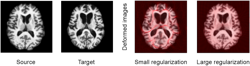
To ensure the smoothness of transformation fields, a regularization term defined on the tangent space of diffeomorphisms (called velocity fields) is often introduced in registration models. Having such a regularity with proper model parameters is critical to registration performance because they greatly affect the estimated transformations. Either too large or small-valued regularity can not achieve satisfying registration results (as shown in Fig .1). Models of handling the regularity parameter mainly include (i) direct optimizing a Bayesian model or treating it as a latent variable to integrate out via Expectation Maximization (EM) algorithm (Allassonnière et al., 2007; Allassonnière and Kuhn, 2008; Zhang et al., 2013; Wang and Zhang, 2021), (ii) exhaustive search in the parameter space (Jaillet et al., 2005; Valsecchi et al., 2013; Ruppert et al., 2017), and (iii) utilizing parameter continuation methods (Haber et al., 2000; Haber and Modersitzki, 2006; Mang and Biros, 2015; Mang et al., 2019). Direct optimization approaches define a posterior of transformation fields that includes an image matching term as a likelihood and a regularization as a prior to support the smoothness of transformations (Zöllei et al., 2007; Allassonnière and Kuhn, 2008; Toews and Wells, 2009). Estimating regularization parameters of these models using direct optimization is not straightforward due to the complex structure of the posterior distribution. Simpson et al. infer the level of regularization in small deformation registration model by mean-field VB inference (Jordan et al., 1999), which allows tractable approximation of full Bayesian inference in a hierarchical probabilistic model (Simpson et al., 2012, 2015). However, these aforementioned algorithms are heavily dependent on initializations, and are prone to getting stuck in the local minima of high-dimensional and non-linear functions in the transformation space. A stochastic approximative expectation maximization (SAEM) algorithm (Allassonnière and Kuhn, 2008) was developed to marginalize over the posterior distribution of unknown parameters using a Markov Chain Monte Carlo (MCMC) sampling method. Later, Zhang et al. estimate the model parameters of regularization via a Monte Carlo Expectation Maximization (MCEM) algorithm for unbiased atlas building problem (Zhang et al., 2013). A recent model of Hierarchical Bayesian registration (Wang and Zhang, 2021) further characterizes the regularization parameters as latent variables generated from Gamma distribution, and integrates them out by an MCEM method.
Despite the achievement of the aforementioned methods, estimating the regularization parameter in a high-dimensional and nonlinear space of 3D MRIs (i.e., dimension is typically or higher) inevitably leads to expensive computational cost through iterative optimizations. To address this issue, we present a deep learning approach to fast predict registration parameters. While there exist learning-based registration models for transformations (Krebs et al., 2019; Balakrishnan et al., 2018; Biffi et al., 2020), we are particularly interested in learning the relationship between pairwise images and optimal regularizations of transformations via regression. In order to produce “ground truth” regularization parameters, we first introduce a low-dimensional Bayesian model of image registration to estimate the best regularity from the data itself. Following a recent work of (Wang et al., 2019), we construct a posterior distribution of diffeomorphic transformations entirely in a bandlimited space with much lower dimensions. This greatly reduces the computational cost of data generation in training. The theoretical tools developed in this work are generic to various deformable registration models, e.g, stationary velocity fields that remain constant over time (Arsigny et al., 2006). The model recommends optimal registration parameters for registration in real-time and has great potential in clinical applications (i.e., image-guided navigation system for brain shift compensation during surgery (Luo et al., 2018)). To summarize, our main contributions are three folds:
- •
To the best of our knowledge, we are the first to present a predictive regularization estimation method for diffeomorphic image registration through deep learning.
- •
We develop a low-dimensional Bayesian framework in a bandlimited Fourier space to speed up the training data generation.
- •
Our model significantly speeds up the parameter estimation, while maintaining comparable registration results.
The paper is organized as follows. In sec. 2, we lay out the basics of image registration optimization in the LDDMM framework. In sec. 3.1, we first develop a low-dimensional posterior distribution that is parametrized by bandlimited velocity fields. We then estimate the regularization parameter by maximizing the posterior. In sec. 3.2, we design a deep convolutional neural network that takes an image pair as input and adaptively predicts the optimal smoothness level for registration. In sec. 4, we validate our model on both 2D synthetic data and 3D brain MRI scans.
2 Background: Fast LDDMM With Geodesic Shooting
In this section, we first briefly review a fast image registration algorithm FLASH in the setting of LDDMM with geodesic shooting (Zhang and Fletcher, 2015, 2019). The core idea of the FLASH is to reparameterize diffeomorphic transformations effectively in its tangent space (also known as velocity fields), where the signals are smooth without developing high frequencies in the Fourier space. This allows all computations of the original LDDMM with geodesic shooting (Vialard et al., 2012; Younes et al., 2009) to be carried out in the bandlimited space of velocity fields with much lower dimensions. As a result, the FLASH algorithm significantly speeds up diffeomorphic image registration with little to no loss of accuracy.
2.1 Geodesic Shooting in Fourier Spaces
Given time-dependent velocity field , the diffeomorphism in the finite-dimensional Fourier domain can be computed as
| (1) |
where is a tensor product , representing the Fourier frequencies of a Jacobian matrix . The is a circular convolution with zero padding to avoid aliasing. We truncate the output of the convolution in each dimension to a suitable finite set to avoid the domain growing to infinity.
Geodesic shooting algorithm states that the transformation can be uniquely determined by integrating a partial differential equation with a given initial velocity forward in time. In contrast to the original LDDMM that optimizes over a collection of time-dependent velocity fields, geodesic shooting estimates an optimal initial velocity . In this work, we adopt an efficient variant of geodesic shooting defined in Fourier spaces. We first discretize the Jacobian and divergence operators using finite difference approximations (particularly the central difference scheme) and then compute their Fourier coefficients. Detailed derivations can be found in the appendix section of FLASH (Zhang and Fletcher, 2019). The Fourier representation of the geodesic constraint that satisfies Euler-Poincaré differential (EPDiff) equation is (Zhang and Fletcher, 2015)
| (2) |
where is a symmetric, positive-definite differential operator that is a function of parameter (details are in Sec. 3.1). Here is the inverse operator of , and is the truncated matrix-vector field auto-correlation 111The output signal maintains bandlimited after the auto-correlation operates on zero-padded input signal followed by truncating it back to the bandlimited space.. The is an adjoint operator to the negative Jacobi–Lie bracket of vector fields, . The operator is the discrete divergence (computed by summing the Fourier coefficients of different directions over in ) of a vector field.
2.2 FLASH: Fast Image Registration
Consider a source image and a target image as square-integrable functions defined on a torus domain (). The problem of diffeomorphic image registration is to find the geodesic (shortest path) of diffeomorphic transformations , such that the deformed image at time point is similar to .
The objective function can be formulated as a dissimilarity term plus a regularization that enforces the smoothness of transformations
| (3) |
The is a distance function that measures the dissimilarity between images. Commonly used distance metrics include sum-of-squared difference ( norm) of image intensities (Beg et al., 2005), normalized cross-correlation (NCC) (Avants et al., 2008), and mutual information (MI) (Wells III et al., 1996). The denotes the inverse of deformation that warps the source image in the spatial domain when . Here is a weight parameter balancing between the distance function and regularity term. The distance term stays in the full spatial domain, while the regularity term is computed in bandlimited space.
3 Our Model: Deep Learning for Regularity Estimation in Image Registration
In this section, we present a supervised learning model based on CNN to predict the regularity of image registration for a given image pair. Analogous to (Yang et al., 2017), we run optimization-based image registration to obtain training data. We introduce a low-dimensional Bayesian model of image registration to produce appropriate regularization parameters for training.
3.1 Low-dimensional Bayesian Model of Registration
In contrast to previous approaches, our proposed model is parameterized in a bandlimited velocity space , with parameter enforcing the smoothness of transformations.
Assuming an independent and identically distributed (i.i.d.) Gaussian noise on image intensities, we obtain the likelihood
| (4) |
where is the noise variance and is the number of image voxels. The deformation corresponds to in Fourier space via the Fourier transform , or its inverse . The likelihood is defined by the residual error between a target image and a deformed source at time point . We assume the definition of this distribution is after the fact that the transformation field is observed through geodesic shooting; hence is not dependent on the regularization parameters.
Analogous to (Wang et al., 2018), we define a prior on the initial velocity field as a complex multivariate Gaussian distribution, i.e.,
| (5) |
where is matrix determinant. The Fourier coefficients of is, i.e., , . Here denotes a negative discrete Fourier Laplacian operator with a -dimensional frequency vector , where is the dimension of the bandlimited Fourier space.
Combining the likelihood in Eq. (4) and prior in Eq. (5) together, we obtain the negative log posterior distribution on the deformation parameter parameterized by as
| (6) |
Next, we optimize Eq. (6) over the regularization parameter and the registration parameter by maximum a posterior (MAP) estimation using gradient descent algorithm. Other optimization schemes, such as BFGS (Polzin et al., 2016), or the Gauss-Newton method (Ashburner and Friston, 2011) can also be applied.
Gradient of . To simplify the notation, first we define . Since the discrete Laplacian operator is a diagonal matrix in Fourier space, its determinant can be computed as . Therefore, the log determinant of operator is
We then derive the gradient term as
| (7) |
Gradient of . We compute the gradient with respect to by using a forward-backward sweep approach developed in (Zhang et al., 2017). Steps for obtaining the gradient are as follows:
- (i)
Forward integrating the geodesic shooting equation Eq.(2) to compute ,
- (ii)
Compute the gradient of the energy function Eq. (3) with respect to at ,
(8) - (iii)
Bring the gradient back to by integrating adjoint Jacobi fields backward in time (Zhang et al., 2017),
(9) where are introduced adjoint variables with an initial condition at .
A summary of the optimization is in Alg. 1. It is worthy to mention that our low-dimensional Bayesian framework developed in bandlimited space dramatically speeds up the computational time of generating training regularity parameters by approximately ten times comparing with high-dimensional frameworks.
3.2 Network Architecture
Now we are ready to introduce our network architecture by using the estimated and given image pairs as input training data. Fig. 2 shows an overview flowchart of our proposed learning model. With the optimal registration regularization parameter obtained from an image pair (as described in Sec. 3.1), a two-stream CNN-based regression network takes source images, target images as training data to produce a predictive regularization parameter. We optimize the network with the followed objective function,
where denotes the regularization on convolution kernel weights . denotes the data fitting term between the ground truth and the network output. In our model, we use norm for both terms. Other network architectures, e.g. 3D Residual Networks (3D-ResNet) (Hara et al., 2017) and Very Deep Convolutional Networks (3D-VGGNet) (Simonyan and Zisserman, 2014; Yang et al., 2018) can be easily applied as well.
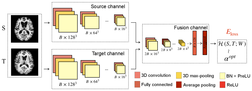
In our network, we input the 3D source and target images into separate channels that include four convolutional blocks. Each 3D convolutional block is composed of a 3D convolutional layer, a batch normalization (BN) layer with activation functions (PReLU or ReLU), and a 3D max-pooling layer. Specifically, we apply convolutional kernel and max-pooling layer to encode a batch (size as ) of source and target images () to feature maps (). After extracting the deep features from source and target channels, we combine them into a fusion channel, which includes three convolutional blocks, a fully connected layer, and an average pooling layer to produce the network output.
4 Experiment
To demonstrate the effectiveness of the proposed low-dimensional Bayesian registration model, we validate it through three sets of experiments. For 2D synthetic data registration, we deform a binary source image with velocity fields sampled from the prior distribution in Eq. (5) with known regularization parameters to simulate target images. We show three convergence graphs of our MAP estimation and compare them with the ground truth parameters.
Similarly, we synthesize image pairs using regularization parameters at different scales respectively, i.e., , to test the performance of our predictive model. We then use the predicted parameter to run registration model and show the error maps between target and deformed images.
For 3D brain MRI registration, we show results on both MAP and our network prediction. We first show the numerical difference between the MAP estimation and our prediction (i.e. predicted regularization parameter), and then report the mean error of deformed images between both methods across all datasets. We visualize the transformation grids and report the value of regularization parameters for both methods. To further investigate the accuracy of parameters generated by our model, we perform registration-based segmentation and examine the resulting segmentation accuracy over nine brain structures, including cortex, putamen, cerebellum, caudate, gyrus, brain stem, precuneus, cuneus, and hippocampus. We evaluate a volume-overlapping similarity measurement, also known as SrensenDice coefficient (Dice, 1945), between the propagated segmentation and the manual segmentation. The statistics of dice evaluation over registration pairs are reported.
We last compare the computational efficiency on both time and memory consumption of the proposed method with a baseline model that performs Bayesian estimation of regularization parameter in the full spatial domain (Zhang et al., 2013).
To generate the training data of initial velocities, we run the proposed low-dimensional Bayesian registration algorithms until convergence. We use the Euler integrator in geodesic shooting and set the of integration steps as . We set algorithm stop rate as and minimal convergence iteration as 30. We use optimal truncated dimension for as 16 and according to (Zhang et al., 2017). For the network setting, We initialize the convolution kernel weights using the He normal initializer (He et al., 2015) and use the Adam optimizer with a learning rate of until convergence. We set and as batch size and weight decay. The maximum epoch for 2D and 3D network training is .
4.1 Data
We run experiments on both 2D synthetic dataset and 3D real brain MRI scans.
2D synthetic data. We generate synthetic bull-eye images with the size of (as shown in Fig. 3). We manipulate the width and height of two ellipses by using equation .
3D brain MRIs. We include public T1-weighted brain MRI scans from Alzheimer’s Disease Neuroimaging Initiative (ADNI) dataset (Jack Jr et al., 2008), Open Access Series of Imaging Studies (OASIS) (Fotenos et al., 2005), and LONI Probabilistic Brain Atlas Individual Subject Data (LPBA40) (Shattuck et al., 2008), among which subjects have manual delineated segmentation labels. All 3D data were carefully pre-processed as , isotropic voxels, and underwent skull-stripped, intensity normalized, bias field corrected, and pre-aligned with affine transformation.
For both 2D and 3D datasets, we split the images by using as training images, as validation images, and as testing images such that no subjects are shared across the training, validation, and testing stage. We evaluate the hyperparameters of models and generate preliminary experiments on the validation dataset. The testing set is only used for computing the final results.
4.2 Results
Fig. 3 displays our MAP estimation of registration results including appropriate regularity parameters on 2D synthetic images. The middle panel of Fig. 3 reports the convergence of estimation vs. ground truth. It indicates that our low-dimensional Bayesian model provides trustworthy regularization parameters that are fairly close to ground truth for network training. The bottom panel of Fig. 3 shows the convergence graph of the total energy for our MAP approach.
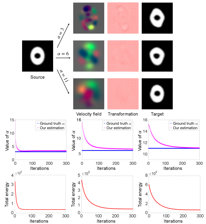
Fig. 4 further investigates the consistency of our network prediction. The left panel shows estimates of regularization parameter at multiple scales, i.e., , over 2D synthetic image pairs respectively. The right panel shows the mean error of image differences between deformed source images by transformations with predicted and target images. While there are small variations on estimated regularization parameters, the registration results are very close (with averaged error at the level of ).
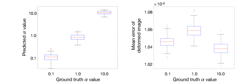
Fig. 5 shows examples of 2D pairwise image registration with regularization estimated by MAP and our predictive deep learning model. We obtain the regularization parameter (MAP) vs. (network prediction), and (MAP) vs. (network prediction). The error map of deformed images indicates that both estimations obtain fairly close registration results.
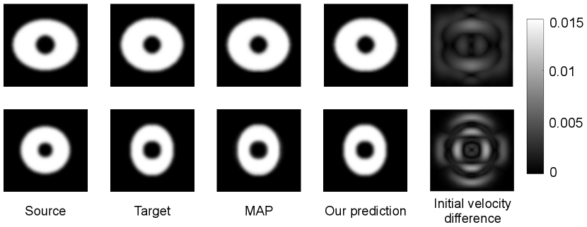
Fig. 6 displays deformed 3D brain images overlaid with transformation grids for both methods. The parameter estimated from our model produces a comparable registration result. From our observation, a critical pattern between the optimal and its associate image pairs is that the value of is relatively smaller when large deformation occurs. This is because the image matching term (encoded in the likelihood) requires a higher weight to deform the source image.
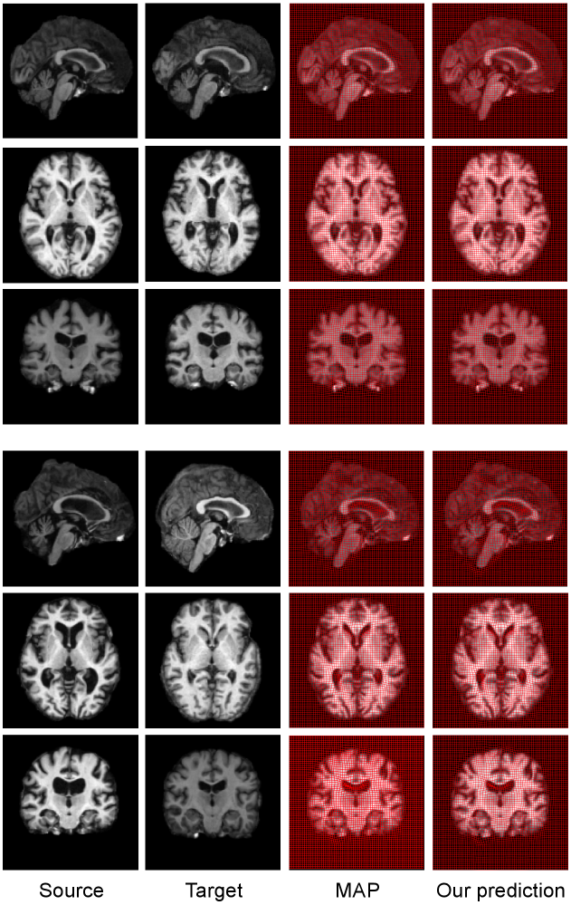
Fig. 7 investigates the consistency of our network prediction over three different datasets of 3D brain MRI. The left panel shows the absolute value of numerical differences between predicted regularization parameters and MAP estimations. The right panel shows the voxel-wise mean error of image differences between deformed images by transformations with predicted and deformed images by MAP. While slight numerical difference on estimated regularization parameters exists, the 3D deformed images are fairly close (with averaged voxel-wise error at the level of ).
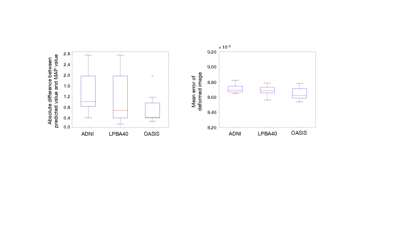
Fig. 8 visualizes three views of the deformed brain images (overlay with propagated segmentation label) that are registered by MAP and our prediction. Our method produces a registration solution, which is highly close to the one estimated by MAP. The propagated segmentation label fairly aligns with the target delineation for each anatomical structure. While we show different views of 2D slices of brains, all computations are carried out fully in 3D.

Fig. 9 reports the volume overlapping of nine anatomical structures for both methods, including Cor(cortex), Puta (putamen), Cere (cerebellum), Caud (caudate), gyrus, Stem (brain stem), Precun (precuneus), Cun (cuneus), and Hippo (hippocampus). Our method produces comparable dice scores comparing with MAP estimations. This indicates that the segmentation-based registration by using our estimation achieves comparable registration performance with little to no loss of accuracy.
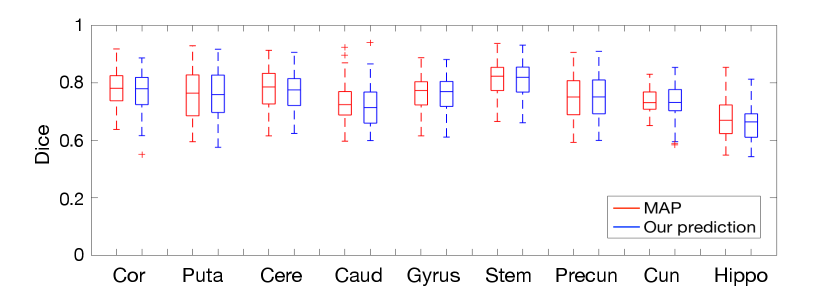
Table. 1 quantitatively reports the averaged time and memory consumption of MAP estimation in full spatial image domain and our method. The proposed predictive model provides appropriate regularization parameters approximately times faster than the conventional optimization-based registration method with a much lower memory footprint.
| Methods | Full-spatial MAP | Low-dimensional MAP | Network Prediction |
|---|---|---|---|
| Runtime (Sec) | 1901 | 257 | 2.16 |
| Memory (MB) | 450 | 119 | 34.4 |
5 Conclusion
In this paper, we proposed a deep learning-based approach to model the relationship between the regularization of image registration and the input image data. We first developed a low-dimensional Bayesian model that defines image registration entirely in a bandlimited space. We then learned the mapping between regularization parameters and spatial images through a CNN-based neural network. To the best of our knowledge, we are the first to predict the optimal regularization parameter of diffeomorphic image registration by deep learning approaches. In contrast to existing methods, our developed model substantially improves the efficiency and the robustness of image registration. Our work has great potential in a variety of clinical applications, e.g. image-guided navigation system for neurosurgery in real-time. Potential future work may include: i) extending the current model to further consider adversarial examples, i.e., image outliers with significant differences; and ii) developing an unsupervised learning of registration parameter estimation to eliminate the need of training data generation (ground truth labels).
Acknowledgments
This work was supported by a startup funding at the University of Virginia.
Ethical Standards
The work follows appropriate ethical standards in conducting research and writing the manuscript, following all applicable laws and regulations regarding treatment of animals or human subjects.
References
- Allassonnière and Kuhn (2008) Stéphanie Allassonnière and Estelle Kuhn. Stochastic algorithm for parameter estimation for dense deformable template mixture model. arXiv preprint arXiv:0802.1521, 2008.
- Allassonnière et al. (2007) Stéphanie Allassonnière, Yali Amit, and Alain Trouvé. Towards a coherent statistical framework for dense deformable template estimation. Journal of the Royal Statistical Society: Series B (Statistical Methodology), 69(1):3–29, 2007.
- Arsigny et al. (2006) Vincent Arsigny, Olivier Commowick, Xavier Pennec, and Nicholas Ayache. A log-euclidean framework for statistics on diffeomorphisms. In International Conference on Medical Image Computing and Computer-Assisted Intervention, pages 924–931. Springer, 2006.
- Ashburner and Friston (2005) John Ashburner and Karl Friston. Unified segmentation. Neuroimage, 26(3):839–851, 2005.
- Ashburner and Friston (2011) John Ashburner and Karl J Friston. Diffeomorphic registration using geodesic shooting and gauss–newton optimisation. NeuroImage, 55(3):954–967, 2011.
- Avants et al. (2008) Brian B Avants, Charles L Epstein, Murray Grossman, and James C Gee. Symmetric diffeomorphic image registration with cross-correlation: evaluating automated labeling of elderly and neurodegenerative brain. Medical image analysis, 12(1):26–41, 2008.
- Balakrishnan et al. (2018) Guha Balakrishnan, Amy Zhao, Mert R Sabuncu, John Guttag, and Adrian V Dalca. An unsupervised learning model for deformable medical image registration. In Proceedings of the IEEE conference on computer vision and pattern recognition, pages 9252–9260, 2018.
- Beg et al. (2005) MIRZA Faisal Beg, Michael I Miller, Alain Trouvé, and Laurent Younes. Computing large deformation metric mappings via geodesic flows of diffeomorphisms. International journal of computer vision, 61(2):139–157, 2005.
- Biffi et al. (2020) Carlo Biffi, Juan J Cerrolaza, Giacomo Tarroni, Wenjia Bai, Antonio De Marvao, Ozan Oktay, Christian Ledig, Loic Le Folgoc, Konstantinos Kamnitsas, Georgia Doumou, et al. Explainable anatomical shape analysis through deep hierarchical generative models. IEEE transactions on medical imaging, 39(6):2088–2099, 2020.
- De Craene et al. (2012) Mathieu De Craene, Gemma Piella, Oscar Camara, Nicolas Duchateau, Etelvino Silva, Adelina Doltra, Jan D’hooge, Josep Brugada, Marta Sitges, and Alejandro F Frangi. Temporal diffeomorphic free-form deformation: Application to motion and strain estimation from 3d echocardiography. Medical image analysis, 16(2):427–450, 2012.
- Dice (1945) Lee R Dice. Measures of the amount of ecologic association between species. Ecology, 26(3):297–302, 1945.
- Fotenos et al. (2005) Anthony F Fotenos, AZ Snyder, LE Girton, JC Morris, and RL Buckner. Normative estimates of cross-sectional and longitudinal brain volume decline in aging and ad. Neurology, 64(6):1032–1039, 2005.
- Gao et al. (2016) Yang Gao, Miaomiao Zhang, Karen Grewen, P Thomas Fletcher, and Guido Gerig. Image registration and segmentation in longitudinal mri using temporal appearance modeling. In 2016 IEEE 13th International Symposium on Biomedical Imaging (ISBI), pages 629–632. IEEE, 2016.
- Haber and Modersitzki (2006) Eldad Haber and Jan Modersitzki. A multilevel method for image registration. SIAM journal on scientific computing, 27(5):1594–1607, 2006.
- Haber et al. (2000) Eldad Haber, Uri M Ascher, and Doug Oldenburg. On optimization techniques for solving nonlinear inverse problems. Inverse problems, 16(5):1263, 2000.
- Hara et al. (2017) Kensho Hara, Hirokatsu Kataoka, and Yutaka Satoh. Learning spatio-temporal features with 3d residual networks for action recognition. In Proceedings of the IEEE International Conference on Computer Vision Workshops, pages 3154–3160, 2017.
- He et al. (2015) Kaiming He, Xiangyu Zhang, Shaoqing Ren, and Jian Sun. Delving deep into rectifiers: Surpassing human-level performance on imagenet classification. In Proceedings of the IEEE international conference on computer vision, pages 1026–1034, 2015.
- Hong et al. (2017) Yi Hong, Polina Golland, and Miaomiao Zhang. Fast geodesic regression for population-based image analysis. In International Conference on Medical Image Computing and Computer-Assisted Intervention, pages 317–325. Springer, 2017.
- Jack Jr et al. (2008) Clifford R Jack Jr, Matt A Bernstein, Nick C Fox, Paul Thompson, Gene Alexander, Danielle Harvey, Bret Borowski, Paula J Britson, Jennifer L. Whitwell, Chadwick Ward, et al. The alzheimer’s disease neuroimaging initiative (adni): Mri methods. Journal of Magnetic Resonance Imaging: An Official Journal of the International Society for Magnetic Resonance in Medicine, 27(4):685–691, 2008.
- Jaillet et al. (2005) Léonard Jaillet, Anna Yershova, Steven M La Valle, and Thierry Siméon. Adaptive tuning of the sampling domain for dynamic-domain rrts. In 2005 IEEE/RSJ International Conference on Intelligent Robots and Systems, pages 2851–2856. IEEE, 2005.
- Jordan et al. (1999) Michael I Jordan, Zoubin Ghahramani, Tommi S Jaakkola, and Lawrence K Saul. An introduction to variational methods for graphical models. Machine learning, 37(2):183–233, 1999.
- Krebs et al. (2019) Julian Krebs, Hervé Delingette, Boris Mailhé, Nicholas Ayache, and Tommaso Mansi. Learning a probabilistic model for diffeomorphic registration. IEEE transactions on medical imaging, 38(9):2165–2176, 2019.
- Liao et al. (2016) Ruizhi Liao, Esra A Turk, Miaomiao Zhang, Jie Luo, P Ellen Grant, Elfar Adalsteinsson, and Polina Golland. Temporal registration in in-utero volumetric mri time series. In International Conference on Medical Image Computing and Computer-Assisted Intervention, pages 54–62. Springer, 2016.
- Luo et al. (2018) Jie Luo, Matt Toews, Ines Machado, Sarah Frisken, Miaomiao Zhang, Frank Preiswerk, Alireza Sedghi, Hongyi Ding, Steve Pieper, Polina Golland, et al. A feature-driven active framework for ultrasound-based brain shift compensation. arXiv preprint arXiv:1803.07682, 2018.
- Mang and Biros (2015) Andreas Mang and George Biros. An inexact newton–krylov algorithm for constrained diffeomorphic image registration. SIAM journal on imaging sciences, 8(2):1030–1069, 2015.
- Mang et al. (2019) Andreas Mang, Amir Gholami, Christos Davatzikos, and George Biros. Claire: A distributed-memory solver for constrained large deformation diffeomorphic image registration. SIAM Journal on Scientific Computing, 41(5):C548–C584, 2019.
- Polzin et al. (2016) Thomas Polzin, Marc Niethammer, Mattias P Heinrich, Heinz Handels, and Jan Modersitzki. Memory efficient lddmm for lung ct. In International Conference on Medical Image Computing and Computer-Assisted Intervention, pages 28–36. Springer, 2016.
- Rueckert et al. (2006) Daniel Rueckert, Paul Aljabar, Rolf A Heckemann, Joseph V Hajnal, and Alexander Hammers. Diffeomorphic registration using b-splines. In International Conference on Medical Image Computing and Computer-Assisted Intervention, pages 702–709. Springer, 2006.
- Ruppert et al. (2017) Guilherme CS Ruppert, Giovani Chiachia, Felipe PG Bergo, Fernanda O Favretto, Clarissa L Yasuda, Anderson Rocha, and Alexandre X Falcão. Medical image registration based on watershed transform from greyscale marker and multi-scale parameter search. Computer Methods in Biomechanics and Biomedical Engineering: Imaging & Visualization, 5(2):138–156, 2017.
- Shattuck et al. (2008) David W Shattuck, Mubeena Mirza, Vitria Adisetiyo, Cornelius Hojatkashani, Georges Salamon, Katherine L Narr, Russell A Poldrack, Robert M Bilder, and Arthur W Toga. Construction of a 3d probabilistic atlas of human cortical structures. Neuroimage, 39(3):1064–1080, 2008.
- Simonyan and Zisserman (2014) Karen Simonyan and Andrew Zisserman. Very deep convolutional networks for large-scale image recognition. arXiv preprint arXiv:1409.1556, 2014.
- Simpson et al. (2012) Ivor JA Simpson, Julia A Schnabel, Adrian R Groves, Jesper LR Andersson, and Mark W Woolrich. Probabilistic inference of regularisation in non-rigid registration. NeuroImage, 59(3):2438–2451, 2012.
- Simpson et al. (2015) Ivor JA Simpson, Manuel Jorge Cardoso, Marc Modat, David M Cash, Mark W Woolrich, Jesper LR Andersson, Julia A Schnabel, Sébastien Ourselin, Alzheimer’s Disease Neuroimaging Initiative, et al. Probabilistic non-linear registration with spatially adaptive regularisation. Medical image analysis, 26(1):203–216, 2015.
- Toews and Wells (2009) Matthew Toews and William M Wells. Bayesian registration via local image regions: information, selection and marginalization. In International Conference on Information Processing in Medical Imaging, pages 435–446. Springer, 2009.
- Vaillant et al. (2004) Marc Vaillant, Michael I Miller, Laurent Younes, and Alain Trouvé. Statistics on diffeomorphisms via tangent space representations. NeuroImage, 23:S161–S169, 2004.
- Valsecchi et al. (2013) Andrea Valsecchi, Jérémie Dubois-Lacoste, Thomas Stützle, Sergio Damas, José Santamaria, and Linda Marrakchi-Kacem. Evolutionary medical image registration using automatic parameter tuning. In 2013 IEEE Congress on Evolutionary Computation, pages 1326–1333. IEEE, 2013.
- Vialard et al. (2012) François-Xavier Vialard, Laurent Risser, Daniel Rueckert, and Colin J Cotter. Diffeomorphic 3d image registration via geodesic shooting using an efficient adjoint calculation. International Journal of Computer Vision, 97(2):229–241, 2012.
- Wang and Zhang (2021) Jian Wang and Miaomiao Zhang. Bayesian atlas building with hierarchical priors for subject-specific regularization. arXiv e-prints, pages arXiv–2107, 2021.
- Wang et al. (2018) Jian Wang, William M Wells, Polina Golland, and Miaomiao Zhang. Efficient laplace approximation for bayesian registration uncertainty quantification. In International Conference on Medical Image Computing and Computer-Assisted Intervention, pages 880–888. Springer, 2018.
- Wang et al. (2019) Jian Wang, William M Wells III, Polina Golland, and Miaomiao Zhang. Registration uncertainty quantification via low-dimensional characterization of geometric deformations. Magnetic Resonance Imaging, 64:122–131, 2019.
- Wells III et al. (1996) William M Wells III, Paul Viola, Hideki Atsumi, Shin Nakajima, and Ron Kikinis. Multi-modal volume registration by maximization of mutual information. Medical image analysis, 1(1):35–51, 1996.
- Xing et al. (2019) Jiarui Xing, Ulugbek Kamilov, Wenjie Wu, Yong Wang, and Miaomiao Zhang. Plug-and-play priors for reconstruction-based placental image registration. In Smart Ultrasound Imaging and Perinatal, Preterm and Paediatric Image Analysis, pages 133–142. Springer, 2019.
- Yang et al. (2018) Chengliang Yang, Anand Rangarajan, and Sanjay Ranka. Visual explanations from deep 3d convolutional neural networks for alzheimer’s disease classification. In AMIA Annual Symposium Proceedings, volume 2018, page 1571. American Medical Informatics Association, 2018.
- Yang et al. (2017) Xiao Yang, Roland Kwitt, Martin Styner, and Marc Niethammer. Quicksilver: Fast predictive image registration–a deep learning approach. NeuroImage, 158:378–396, 2017.
- Younes et al. (2009) Laurent Younes, Felipe Arrate, and Michael I Miller. Evolutions equations in computational anatomy. NeuroImage, 45(1):S40–S50, 2009.
- Zhang and Fletcher (2015) Miaomiao Zhang and P Thomas Fletcher. Finite-dimensional lie algebras for fast diffeomorphic image registration. In International Conference on Information Processing in Medical Imaging, pages 249–260. Springer, 2015.
- Zhang and Fletcher (2019) Miaomiao Zhang and P Thomas Fletcher. Fast diffeomorphic image registration via fourier-approximated lie algebras. International Journal of Computer Vision, 127(1):61–73, 2019.
- Zhang et al. (2013) Miaomiao Zhang, Nikhil Singh, and P Thomas Fletcher. Bayesian estimation of regularization and atlas building in diffeomorphic image registration. In International conference on information processing in medical imaging, pages 37–48. Springer, 2013.
- Zhang et al. (2016) Miaomiao Zhang, William M Wells, and Polina Golland. Low-dimensional statistics of anatomical variability via compact representation of image deformations. In International conference on medical image computing and computer-assisted intervention, pages 166–173. Springer, 2016.
- Zhang et al. (2017) Miaomiao Zhang, Ruizhi Liao, Adrian V Dalca, Esra A Turk, Jie Luo, P Ellen Grant, and Polina Golland. Frequency diffeomorphisms for efficient image registration. In International conference on information processing in medical imaging, pages 559–570. Springer, 2017.
- Zöllei et al. (2007) Lilla Zöllei, Mark Jenkinson, Samson Timoner, and William Wells. A marginalized map approach and em optimization for pair-wise registration. In Biennial International Conference on Information Processing in Medical Imaging, pages 662–674. Springer, 2007.