

1 Introduction
In medical imaging, the problem of registering images has been tackled by numerous authors (Sotiras et al., 2013) by registering directly the images, most of the time assuming that both images contain the entire object of interest. When dealing with similar images (e.g. same acquisition modality of a given patient), techniques driven by a distance between voxel intensities (called similarity) usually perform well (Bauer et al., 2021). When more variability in terms of intensity arises, other studies propose feature based methods that match structures of interest such as surfaces, curves or even patches (Jiang et al., 2021), showing better robustness than their intensity based counterparts.
The problem of finding correspondences between these structures has numerous applications such as pattern recognition (Bronstein et al., 2006, 2009; van Kaick et al., 2013), annotation (Mori et al. (2013), Feragen et al. (2015)), and reconstruction (Halimi et al., 2020). In particular, in the field of medical imaging, matching an atlas and a patient’s anatomy (Feragen et al., 2015), or comparing exams of the same patient acquired with different imaging techniques (Bashiri et al., 2018), provide critical information to physicians for both planning and decision making. In practice, it often happens that only part of an object is visible in one of the two modalities (e.g. disease, surgery, multi-modality imaging, noise). When only partial correspondence between the images are present, handling missing structures is often done manually or heuristically.
Cone Beam Computed Tomography (CBCT), for instance, is used during image guided procedures -live- to improve navigation and guidance. Yet, the imaged organs are generally larger than the field of view, while the whole organ such as the liver can be acquired in Computed Tomography (CT) scanners during the disease diagnostic phase.
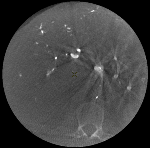
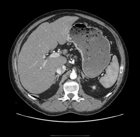
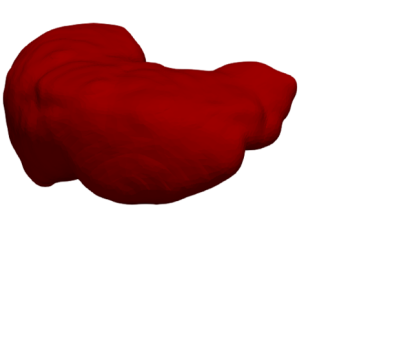
In order to make the best of the different images both in terms of field of view and image characteristics (see Fig. 1), one can find a partial matching between them and the feature-based approaches seem suited to such matching problems. This work is focused on the registration of shapes where only part of these structures can be matched and its application to the registration of liver surfaces extracted from CT and CBCT to guide multi-modal volumes registration. In particular we apply the registration to the whole volumes, and must control the deformations to generate anatomically relevant ones. We study the clinical application of the proposed partial matching term for The present paper is an extension of Antonsanti et al. (2021) from the 2021 Information Processing in Medical Imaging conference in which we introduced the partial matching in the space of varifolds.
1.1 Previous works
The problem of matching shapes has been widely addressed in the literature in the past decades (van Kaick et al., 2011). In the specific case of partial matching, one can find two main approaches to such problem: either by finding correspondences, sparse or dense, between structures from descriptors that are invariant to different transformations (Aiger et al., 2008; Rodolà et al., 2017; Halimi et al., 2019), or by looking for a deformation aligning the shapes with respect to a given metric (Aiger et al., 2008; Mori et al., 2013; Zhao et al., 2015; Feragen et al., 2015; Halimi et al., 2020).
The early works on partial shape correspondence as reviewed in van Kaick et al. (2011) rely on correspondences between points computed from geometric descriptors extracted from an isotropic local region around the selected points. The method is refined in van Kaick et al. (2013) by selecting pairs of points to better fit the local geometry using bilateral map. The features extracted can also be invariant to different transformation, as in Rodolà et al. (2013) where the descriptors extracted are scale invariant. Such sparse correspondences are naturally adapted to partial matching, yet they cannot take the whole shapes into account in the matching process.
Using a different approach, functional maps were introduced in Ovsjanikov et al. (2012) allowing dense correspondences between shapes by transferring the problem to linear functions between spaces of functions defined over the shapes. In Rodolà et al. (2017) the non-rigid partial shape correspondence is based on the Laplace-Beltrami eigenfunctions used as prior in the spectral representation of the shapes. Recently in Halimi et al. (2019), such functional map models were adapted in a deep unsupervised framework by finding correspondences minimizing the distortion between shapes. Such methods are yet limited to surface correspondences.
The second kind of methods relies on the deformations that can be generated to align the shapes with each other. It usually involves minimizing a function called data attachment that quantifies the alignment error between the shapes. A deformation cost is sometimes added to regularize these deformations. The sparse correspondences being naturally suited to partial matching, they are notably used in Iterative Closest Point (ICP) methods and their derivatives to guide a registration of one shape onto the other. In Aiger et al. (2008) a regularized version of the ICP selects the sets of four co-planar points in the points cloud. In Mori et al. (2013) the ICP is adapted to the specific case of vascular trees and compute curves’ correspondences through an Iterative Closest Curve method. Working on trees of 3D curves as well, Feragen et al. (2015) hierarchically selects the overall curves correspondences minimizing the tree space geodesic distance between the trees. This latter method, although specific to tree-structures, allows topological changes in the deformation.
On the other hand some authors compute the deformation guided by a dense data attachment term. In Bronstein et al. (2006) isometry-invariant minimum distortion deformations are applied to 2D Riemannian manifolds thanks to a multiscale framework using partial matching derived from Gromov’s theory. This work is extended in Bronstein et al. (2009) by finding the optimal trade-off between partial shape matching and similarity between these shapes embedded in the same metric space. Recently in Halimi et al. (2020) a partial correspondence is performed through a non-rigid alignment of one shape and its partial scan seen as points clouds embedded in the same representation space. The non-rigid alignment is done with a Siamese architecture network. This approach seems promising and is part of a completion framework, however it requires a huge amount of data to train the network.
Interestingly, the regularization cost can be seen as a distance between shapes itself (Feragen et al., 2015) by quantifying the deformation amount necessary to register one shape onto the other. This provides a complementary tool to the metrics used to quantify the shapes dissimilarities.
A well established and versatile framework to compute meaningful deformations is the Large Deformation Diffeomorphic Metric Mapping (LDDMM) (Trouvé, 1995; Christensen et al., 1996; Beg et al., 2005). It allows to see the difference between shapes through the optimal deformation to register a source shape onto a target shape . However, the data attachment metrics proposed so far aim to compare the source and target shapes in their entirety (Charon et al., 2020), or look for explicit correspondences between subparts of these shapes (Feydy et al., 2017). In Kaltenmark and Trouvé (2018) the proposed growth model introduces a first notion of partial matching incorporated to the LDDMM framework. More recently, the bijectivity constraint is circumvented by the introduction of weighted shapes: in Hsieh and Charon (2021); Sukurdeep et al. (2021), authors optimize a mask defined on the shapes to exclude some subparts of these shapes (source or target). In Antonsanti et al. (2021) a partial matching data fidelity term was introduced in the space of varifolds. We use it in this paper and extend its formulation to better control the non-rigid deformations. We then apply the overall method to guide multi-modal volumes registration.
1.2 Organization of the Paper
In the first part we will shortly review the main elements of the representation of shapes in the space of varifolds (Charon and Trouvé, 2013) and the expression of the partial matching we use in this space, introduced in Antonsanti et al. (2021). In particular, we recall how it can be used with LDDMMs to compute diffeomorphic registration of a source shape to a subset of a target one. We will also discuss the use of the partial matching with a rigid registration. We then provide more details on the regularization term used for the application to the registration of truncated liver surfaces to limit the shrinkage effect that can occur when using partial matching with LDDMM.
The second section of this paper is dedicated to its clinical application to multi-modality volume registration based on the partial matching of liver surfaces. In this application we register liver surfaces obtained from segmentations of pre-interventional CT volumes intended for diagnostic purposes, and per-interventional CBCT volumes in which the livers are wider than the field of view, leading to truncation of the surfaces in the latter modality.
2 Partial Matching in the space of varifolds
In this section we quickly review the methodology introduced in Antonsanti et al. (2021). We refer to this article for all details.
We are interested in the problem of finding an optimal deformation to register a source shape onto an unknown subset of a target shape , where are assumed to be compact -rectifiable subsets of with either (curves) or (hypersurfaces).
2.1 Shape registration via oriented varifolds
The varifold method for shape matching was first introduced in Charon and Trouvé (2013). In this section we use the notations and concepts of the more general oriented varifold framework, developed in Kaltenmark et al. (2017). This framework associates with any shape a representer function, defined on , as follows:
where denotes the unit tangent vector –for curves– or unit normal vector –for hypersurfaces– at point on the shape , and are predefined fixed kernels functions over and . In practice, we use a gaussian kernel , where is a scale parameter, and for the kernel . Mathematically, the product kernel defines a Reproducing Kernel Hilbert Space (RKHS) structure , and corresponds to the Riesz representer of the oriented varifold , associated with , and the space of continuous linear forms on .
The shape matching dissimilarity between and is then the squared -norm between their representers, which is also the squared (dual) norm between their varifolds:
where the scalar product has an explicit form using the kernels:
2.2 Definition of the Partial Matching Dissimilarity
The proposed partial dissimilarity term is designed to look locally at the inclusion of the deformed source shape into the target one, and to compensate (with the function) for the imbalance of weights between the simple shape and the more complex one with a normalization. The following term tends to 0 when the deformed shape is included in the target one (for more details and discussion, see Antonsanti et al. (2021)).
Definition 1.
Let defined as , and denote for , , and . We define the normalized partial matching dissimilarity as follows:
| (1) |
where with small, is used as a smooth approximation of the function.
Discrete formulation
The discrete version of the partial matching dissimilarity can be derived very straightforwardly, following the same discrete setting described in Charon et al. (2020) for varifold matching. We are working with surfaces, seen as triangular meshes with vertices . Each triangle with the vertices of the shape is associated to the center and to the normal vector . The unit normal vector is then . We define similarly the centers of the target shape and their associated normal vectors and unit normal vectors .
The discrete normalized partial matching term is then written as follows:
| (2) |
with .
2.3 Use in the LDDMM setting
In the LDDMM framework Beg et al. (2005), the partial matching problem consists in minimizing
where is the flow of the time-dependent square integrable velocity fields , and is the regularization Hilbert norm over vector fields.
The LDDMM registration procedure is numerically solved via a geodesic shooting algorithm introduced by Miller et al. (2006), optimizing on a set of initial momentum vectors located at the discretization points of the source shape. Implementations of the dissimilarity terms are available on our github repository 111https://github.com/plantonsanti/PartialMatchingVarifolds.
2.4 Use with Rigid Deformations
We can define a second minimization problem for a rigid registration, by minimizing the function:
with a rigid deformation composed of a translation and a rotation.
For any rigid deformation , , and we can thus write in the discrete setting:
We have that is a composition of continuous functions and that : when the translation goes to infinity from the construction of the kernel . We can deduce that for all rigid deformation we have and .
is continuous and bounded over the space of finite dimension of rotations and translations, the minimization problem has a solution.
2.5 Additional a priori
It is known from experiments that the deformations can lead to abnormal shrinkage or stretching of the deformed shapes. This phenomenon comes from two things combined: first, we introduce an attachment term to the data favoring the inclusion of a deformed object in a target, thus an asymmetric term. In the case of non-rigid deformations, there is a multitude of local minima, and this must be controlled with a regularization of the deformations. Second, in the regularization of the LDDMM model (2.3), the deformations tend to shrink the objects along the geodesics, so it is possible that the diffeomorphisms create a shrinkage of the non-realistic source shape. In order to limit this we can add a regularization term in the function to minimize.
2.5.1 Definition
The purpose of this regularization term is to prevent the deformations from shrinking or stretching the source shape. We chose to address it in the shape space of Varifolds as well, by controlling the norm of the deformed shape:
| (3) |
Interestingly this term can be written with the area formula:
This enforces the conservation of the norm of the deformed shape. Yet in practice it can lead to local deformations of one part of the shape compensated with another part (Fig. 2). We therefore introduce a local regularization allowing to locally preserve the mass by enforcing the terms inside the integral to be close to everywhere:
| (4) |
Discrete formulation
Similarly to the partial matching term, we can write the regularization terms (both global and local) in the discrete setting:
| (5) |
| (6) |
The overall function to minimize in this LDDMM setting is given by the formula:
| (7) |
with or .
Proposition 1.
Let and be two fixed parameters. The regularized partial matching problem, which consists in minimizing over the function (defined in Eq.2.5.1) has a solution.
Similarly to Antonsanti et al. (2021), the proof boils down to showing that the mapping is weakly continuous on . We use the same notations, and define a sequence in , weakly converging to some . We only need to show that .
To simplify we denote , and for any , and likewise for .
2.5.2 Influence of the Regularization Term
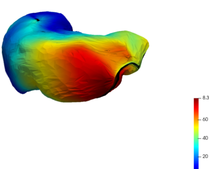
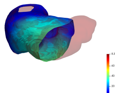
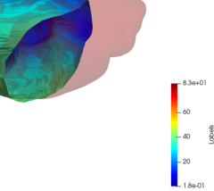
We illustrate the influence of the regularization terms with the example of the registration of a truncated surface onto a complete one. To do so we perform a LDDMM registration using a small regularization parameter in the functional and we set . The data attachment term we use is the one proposed for the partial matching in Section. 2.2.
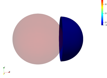
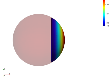
No Regularization
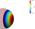
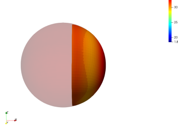
Global Regularization
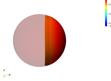
Local Regularization
We observe that without any regularization, the non-rigid deformations lead to global shrinkage of the source shape. On the contrary the proposed regularizations both global and local prevent from such shrinkage. The global one though preserves the norm of the shape at the end of the diffeomorphic deformation and does not prevent from inconsistent local deformations. The most regular deformation is thus induced by the local regularization, which allows to locally control the value of the varifold associated to the deformed source. It should be noted that we work at a small scale of attachment to the data, and that this influences the regularization. In the rest of the paper, we will use this local mass preserving term for the clinical application (section 3).
2.5.3 Implementation Details
In all the following experiments, we initialize the registration by aligning objects barycenters since no prior positioning is known in our applications. To model non-rigid deformations, we define the reproducing kernel of to be a sum of Gaussian kernels:
where and is about half the size of the shapes bounding boxes. For each set of experiments we use the same hyperparameters () to compare the influence of the regularization and for the clinical application. The parameter controls the range of the non-rigid deformations produced by LDDMM, while is associated to the spatial kernel used for the data attachment term in the space of varifolds, and denotes the reach of each varifold. Our Python implementation makes use of the libraries PyTorch (Paszke et al., 2017) and KeOps (Charlier et al., 2021), to benefit from automatic differentiation and GPU acceleration of kernel convolutions.
2.5.4 Computational Cost
To compute the registrations, we use a TITAN RTX Graphic Processing Unit. One rigid deformation of a voxel grid is computed in when the diffeomorphic deformation takes seconds. In terms of optimization, the ICP (on CPU) takes for a source and a target of approximately points. On the same data the rigid registration guided with our partial matching dissimilarity function takes and the LDDMM optimization takes . This huge difference between LDDMM and the others methods comes from the number of parameters to optimize in its framework : the dimension of the space times the number of points in the source shape.
There are many possible ways to accelerate the LDDMM, from reducing the number of points in the source to the approximation of the diffeomorphisms with other deformations models. No matter the deformation, the computational cost of the partial matching dissimilarity function for the same data is .
3 Clinical application : Feature-based Multi-modality Liver Volume Registration
Medical images are often acquired through different modalities, including ultrasound, computed tomography, and magnetic resonance imaging, each providing different and complementary information. In this context, image registration allows physicians to obtain combined inputs from different imaging modalities using for instance image comparison or fusion. The latter has been shown to be valuable in image-guided procedures, yielding less complications and decreasing radiation dose (Rajagopal and Venkatesan, 2016). This section is the clinical application of the work introducing the partial matching in the space of varifolds (Antonsanti et al., 2021) and the extensions proposed in 2.
3.1 CT/CBCT Volume Registration
Transcatheter directed liver therapies are part of the therapeutic arsenal of primary and secondary liver malignancies. The objective of these procedures is to locally treat the tumor and be as selective as possible (meaning placing the microcatheter used to inject the treatment as close as possible to the tumor) to preserve surrounding healthy tissues all while ensuring the destruction of the malignant cells.
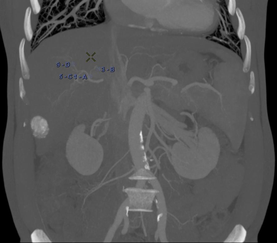
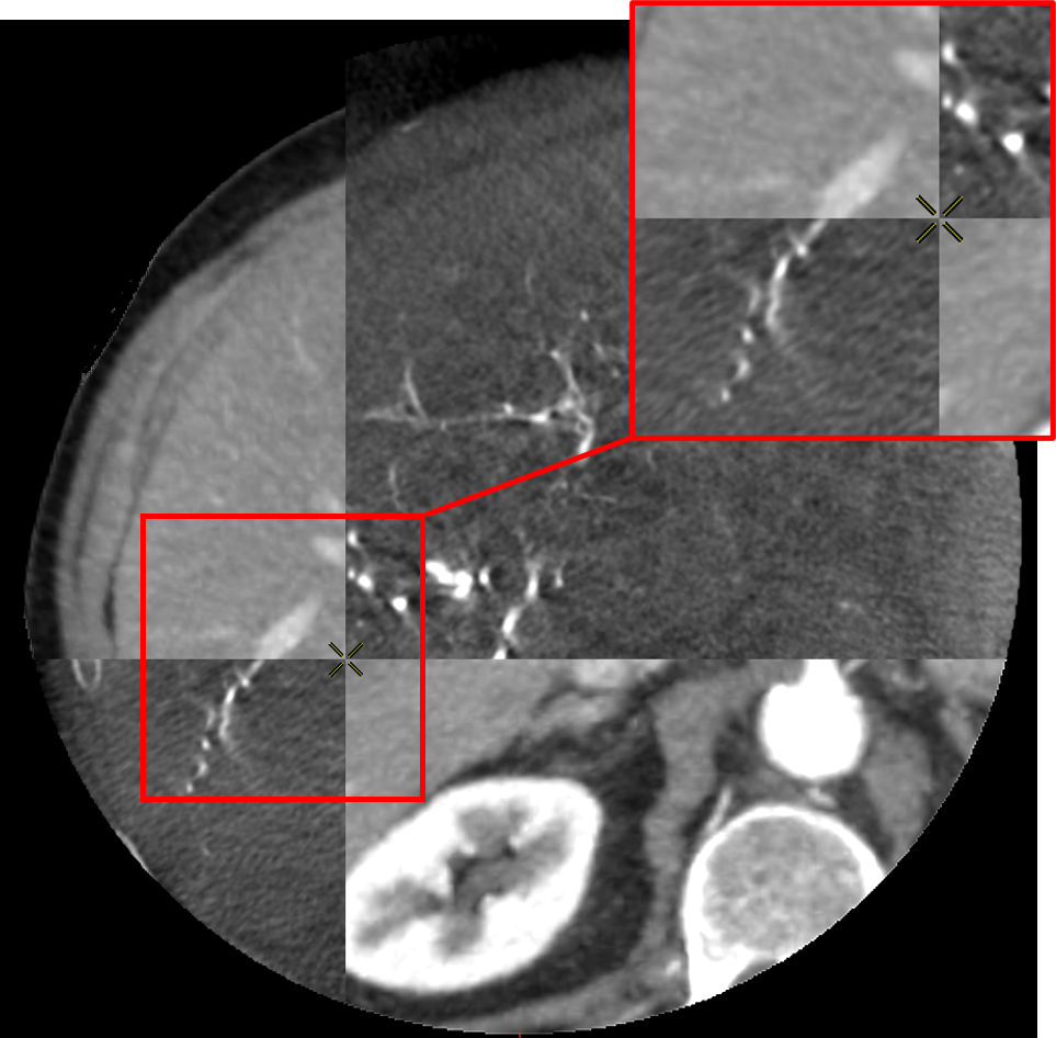
These minimally invasive procedures are performed by navigating through the patient’s arteries under real time 2D angiography, acquired through an imaging device called C-arm. Additionally, the latter can perform a 200 degrees rotation to allow 3D reconstruction of the patient’s anatomy, called Cone Beam Computed Tomography (CBCT) (Tacher et al., 2015), to obtain a “live” 3D imaging of the patient at point of care. Performing CBCT during such procedure improves tumor detection and navigation guidance (Fig. 1a).
Classically, preprocedural diagnostic CT scan or MRI are reviewed by the interventional radiologist to plan the procedure accordingly. The preprocedural acquisitions provide information on the entire liver anatomy, tumor burden and tumor feeding arteries that are decisive for procedural planning, such as number of tumors to be treated in one session and the dose of therapeutic agent to inject. Contrary to CT or MRI, CBCT is performed during the procedure, and the operator can compare procedural CBCT to preprocedural CT (Fig. 1b) to ensure adequate treatment delivery.
While CBCT offers a superior spatial resolution compared to conventional CT scan, with intra-arterial injection of contrast agent providing a detailed visualization of the arteries, low contrast visibility is better in CT (Fig. 1a). CBCT can also be subject to several artifacts such as beam hardening and motion artifacts that might decrease the CBCT performance to visualize the tumor, which is key to selective and successful treatment. A major difficulty in the fusion of a CT volume with a CBCT one comes from the fact that, unlike CT, liver is only partially visible in CBCT (due to the limited size of the field of view in the latter modality). In addition the acquisitions are taken at different times, potentially several weeks apart, and with different patient stances introducing deformations of the liver. For all these reasons, the two types of volumes are very different one from another as illustrated in Fig. 1.
We propose a registration method based on liver surfaces (one of the feature that is visible in both the CT and CBCT whatever the clinical acquisition protocol) providing a deformation of the entire volume. To that extent we apply our partial matching dissimilarity term allowing to tackle the issue of partial correspondence between the truncated surface extracted from the CBCT (Live) and the one extracted from the CT (Liver). The registrations are evaluated on landmarks inside the liver, which were annotated by a physician.
3.2 Database Description
The database is composed of CBCT/CT pairs where CBCT have been acquired during hepatic arteriography and CT scans obtained at early or late arterial phase. We do not provide the acquisition parameters here, yet the spatial resolution (in ) of the volumes are for the CBCT and in average for the CT. Both were selected to show good visualization of the vessels and tumors. In total, 19 pairs of CT/CBCT liver volumes were evaluated, as the one illustrated in Fig. 1.
3.2.1 Liver Segmentation
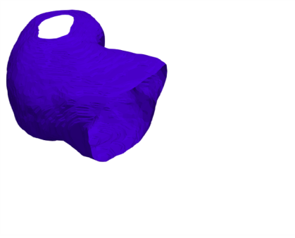
The livers were segmented in each modality using a deep neural network (Milletari et al., 2016) providing a binary volume in both modalities. In this application, the segmentations were evaluated by a clinical specialist and manually corrected if a major error was detected such as missing part of the liver. The idea is to be close to the clinical set up. By doing so, we ensure that the registrations are based on features as reliable as possible. The mesh of the surfaces were then extracted and decimated, leading to meshes of approximately points per surface. In the case of CBCT volumes, the meshes are then cut by the cylinder corresponding to the field of view using Musy et al. (2021). The CBCT livers surfaces obtained are then truncated.
3.2.2 Points of Interest
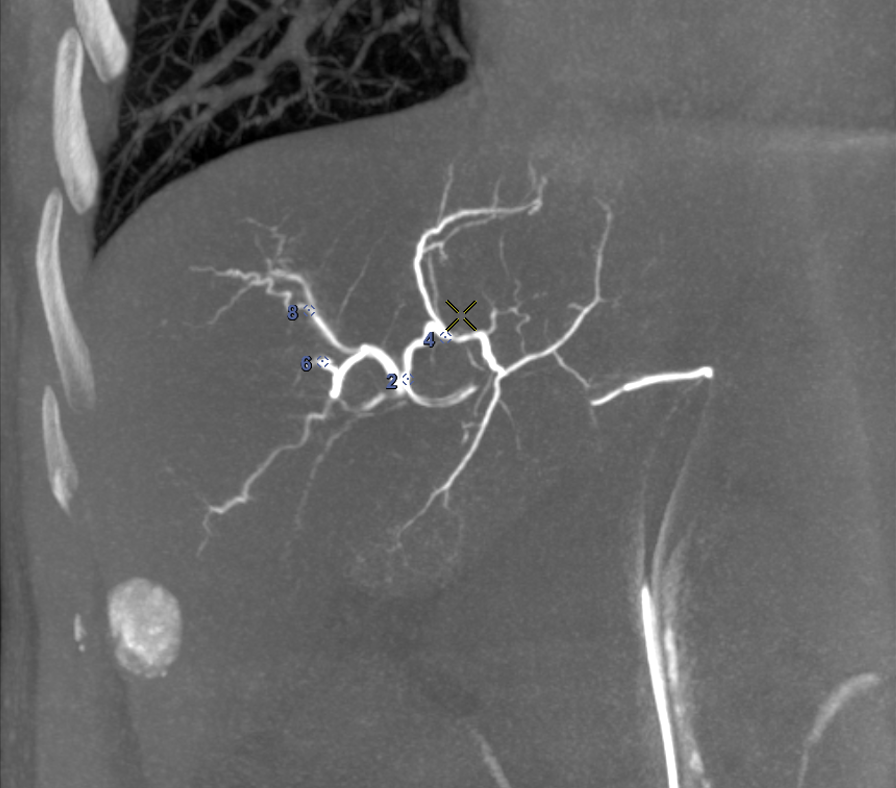
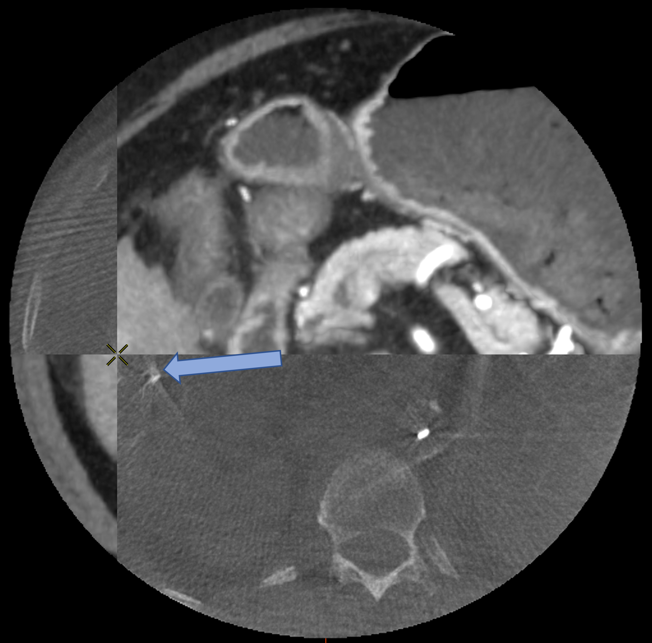
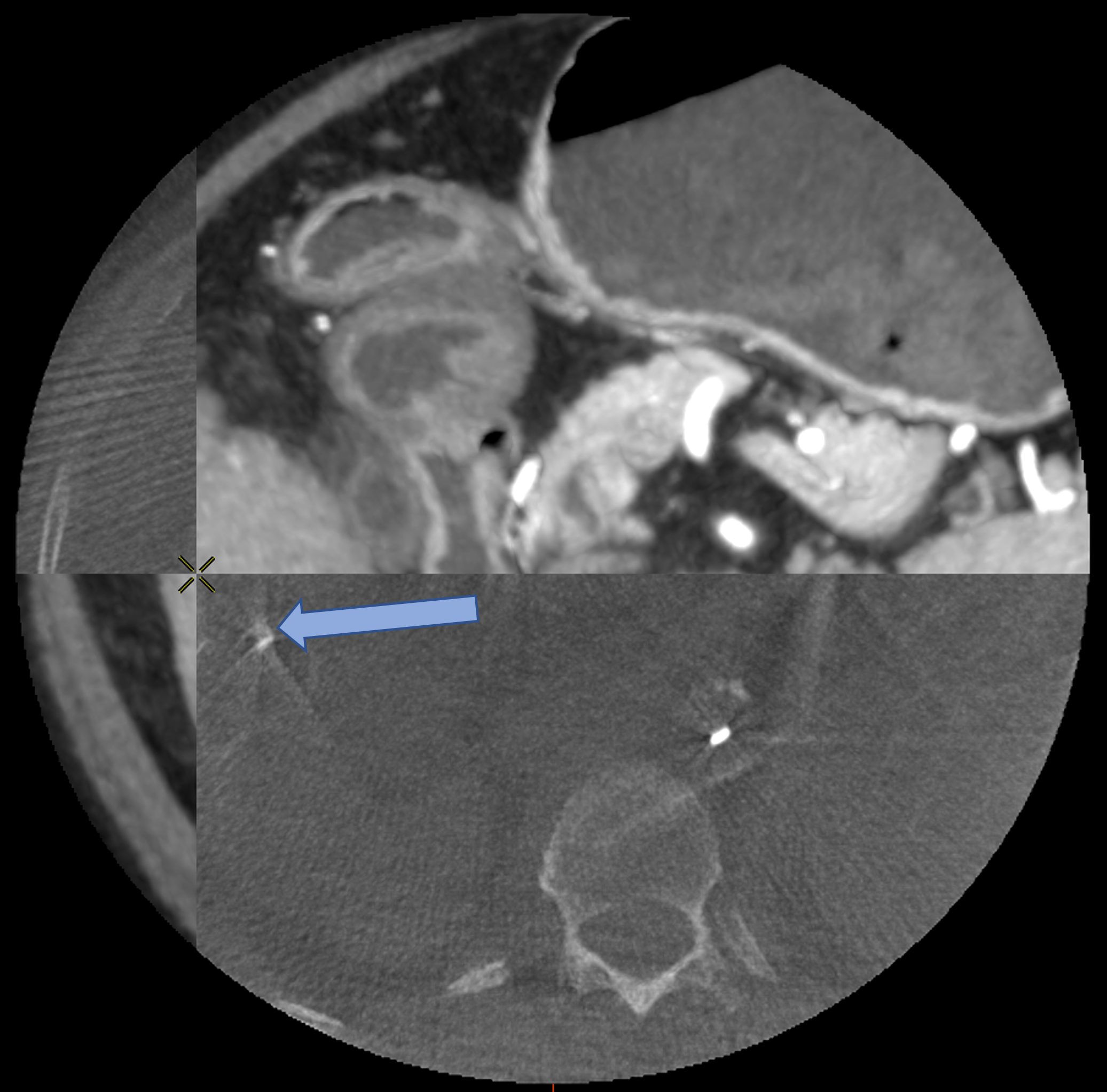
For each patient, the branches of the proper hepatic artery visible on CT volume were annotated with Points of Interest (POIs) for evaluation purpose. Each POI was similarly annotated in the same location on the corresponding CBCT volume. Selected POIs often corresponded to arterial bifurcations that are easily identifiable on both CT and CBCT. For each pair of volumes, a physician annotated 10 POIs (Fig. 3a,3b). Because of the limited visibility of distal hepatic arteries on arterial phase CT compared to CBCT acquired during hepatic arteriography, most of POIs were located close to the bifurcation of the proper hepatic artery, thus mainly located at central parts of the livers, of importance to physicians.
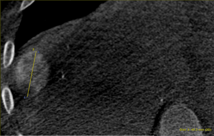
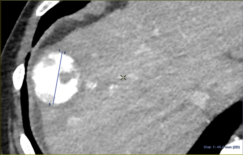
3.2.3 Tumors Annotation
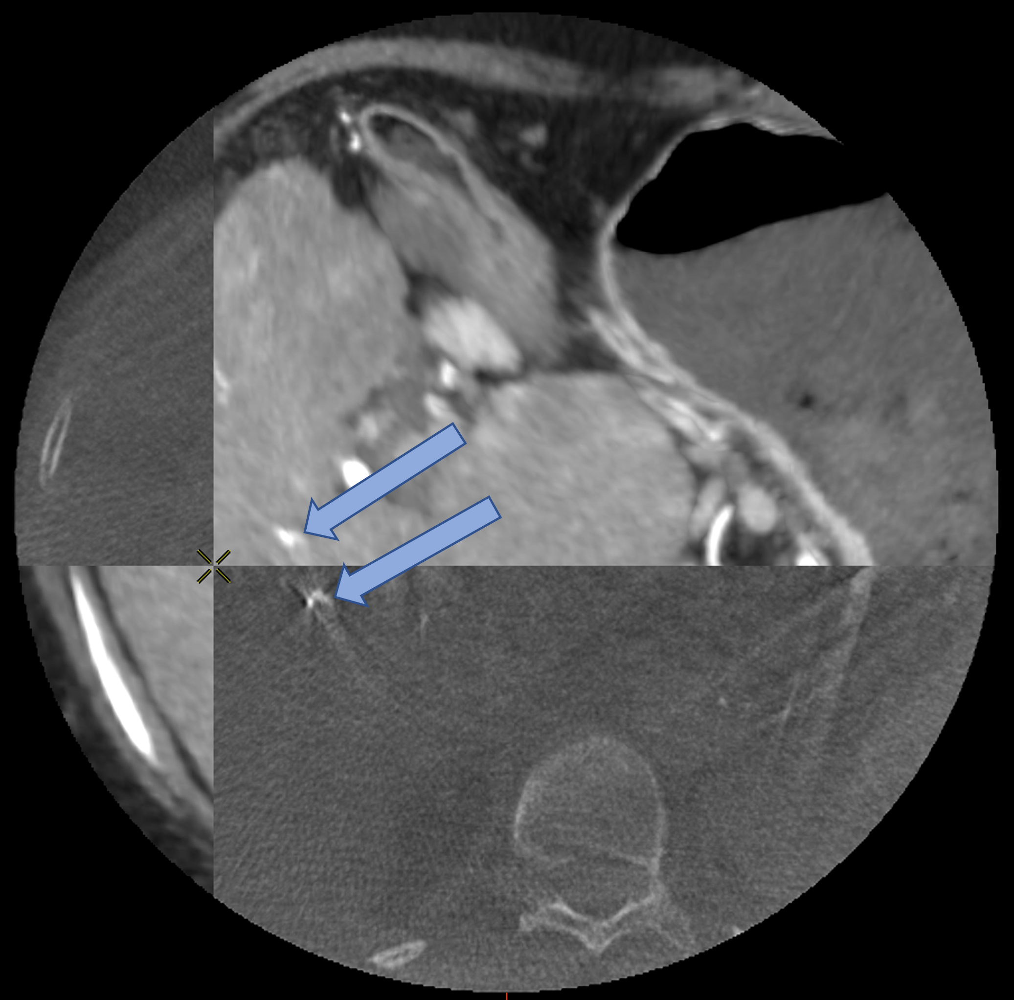
To evaluate the registrations, in addition to POIs, we annotated the longest axis diameter of a tumor according to Ghosn et al. (2021) to ensure better reproducibility of the annotations across volumes (Fig. 3c, Fig 3d). It was done in the axial view of the volumes for tumors that were visible in both modalities. The axis can be decomposed into 3 Tumor Points : the extremities and the center. In the database, one invasive tumor could not be annotated, reducing the number of pairs of tumors to 18. The annotated tumors were located in all the liver segments and their size varied from 9mm to 109mm. This variability in terms of position and size provides a complementary information to that of the POIs.
3.3 Liver Surface Registration with Partial Matching
As a first registration step, the truncated liver surfaces from CBCT were registered onto complete liver surfaces from CT scans with a LDDMM deformation model using the discrete framework described in Sec. 2.2. The LDDMM deformations of the truncated livers surfaces with partial dissimilarity function may lead to small shrinkage of the borders. To compensate this phenomenon in the application we added the a priori regularization of Eq. 4 to the partial data attachment term that prevents from strong local deformations. For illustration purpose, one subject was registered twice with this model: once with the distance in the space of Varifolds, once with the normalized partial dissimilarity term (Def. 1) with the local regularization (Eq. 4). This particular experiment is illustrated in Fig. 4. Both results are generated with the same deformations and regularization parameters. As expected the Varifold distance leads to unrealistic deformations that tend to fill the holes in the source shape to cover the entire target. From the anatomical and medical point of view this is misleading and can not be used in a clinical application of multi-modality volumes registration. On the contrary the partial matching produces a more realistic deformation of the source onto a subset of the complete surface. We will only use and discuss this model in the following.
To initialize the LDDMM deformations, one classically performs a rigid registration. We find in the literature that the livers are principally deformed in translation, so we tested a set of combinations between rigid deformations and LDDMM. We selected the methods providing the best results: a translation followed by LDDMM (denoted translation+LDDMM) and a rigid deformation of limited angulation followed by LDDMM (denoted rigid+LDDMM). The rigid registration is limited to rotations between and around each axis that is the range of realistic rotations for the liver deformations.
In addition to these registration methods, we tested the standard rigid Iterative Closest Point (ICP) applied to the surfaces, using as data attachment term the function:
By minimizing this term one minimizes the average distance of the source points to the target. This asymmetric function can be seen as a partial matching dissimilarity term, being equal to if is included in .
3.3.1 Implementation details
LDDMM is computed with the partial matching dissimilarity term and the localized mass preservation term Eq. 4. In the rest of the paper is written as follows:
| (8) |
The optimization of this functional is performed using Limited-memory Broyden–Fletcher–Goldfarb–Shanno (L-BFGS) algorithm. In the LDDMM framework the cost of the deformations is controlled by the parameters and . To enforce smooth deformations of the surface as well as its ambient space, we set to , and we control the risk of shrinkage of the partial matching non-rigid registration by setting . The Reproducing Kernel of the deformations is the same as in 2.5.3 allowing large deformations of the shapes along with more detailed ones. To better register the shapes, we also use a multi-scale registration scheme for the data attachment terms by iterative applications with and the output of the optimization at scale is used as input at the scale .
3.4 From Surface to Volume Registration
Both rigid deformation and LDDMM can be extended to the whole volume.
Rigid
Rigid+LDDMM
Translation+LDDMM
with ICP
with Partial Varifold
with Partial Varifold
Tumor metric : 9.12mm

Tumor metric : 9.32mm
Tumor metric : 2.86mm
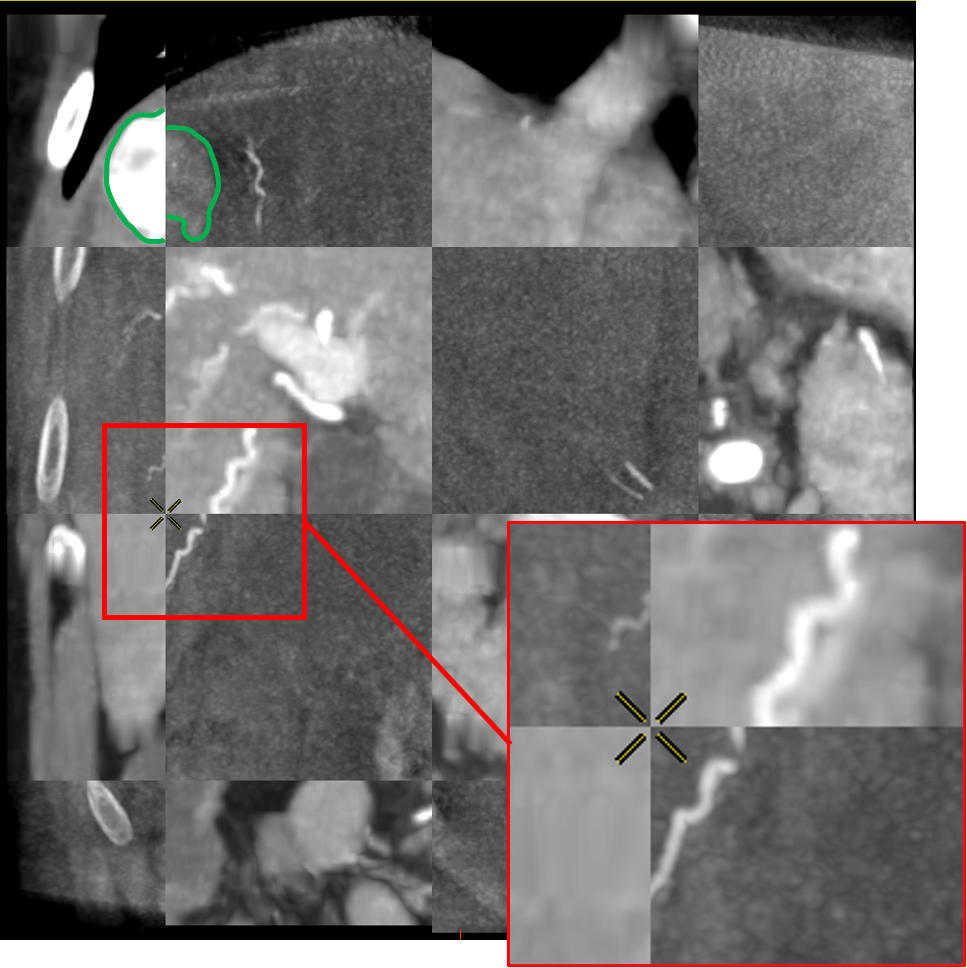
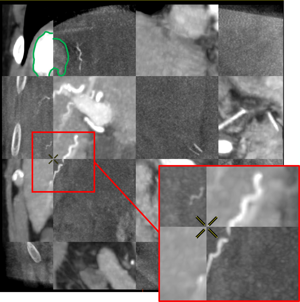
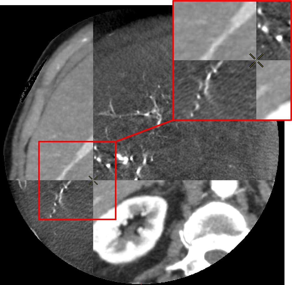
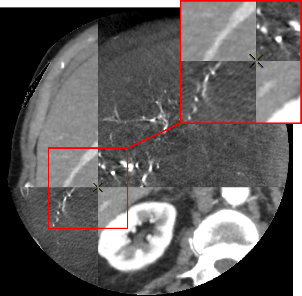
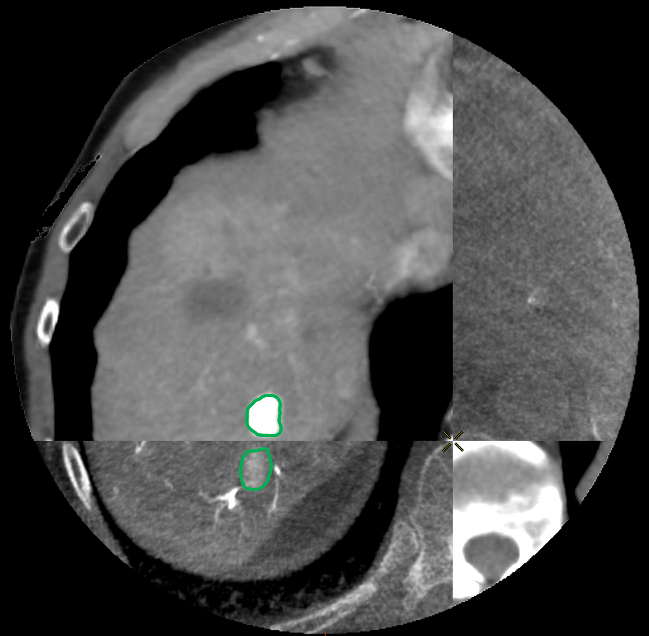
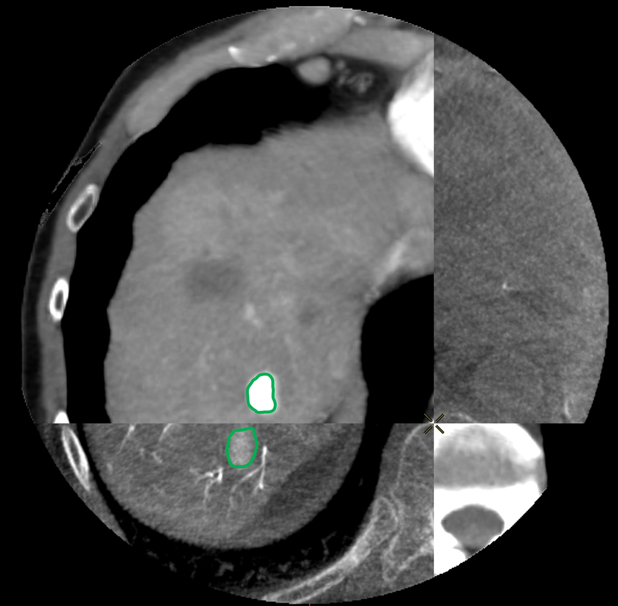
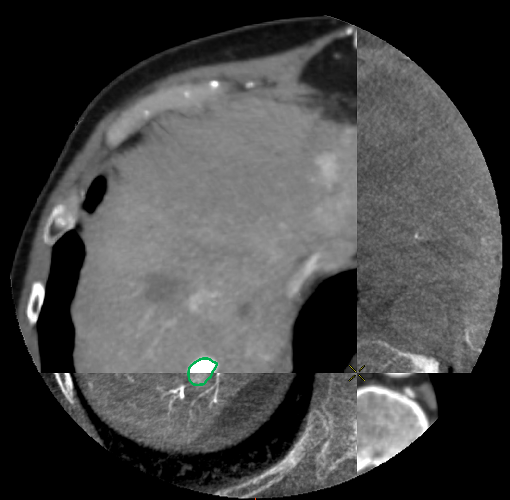
To do so, the voxel grid of the source volume is deformed and interpolated on the target volume. In the case of LDDMM deformations, the voxel grid is deformed with the diffeomorphism of as described in 2.3. The values of the interpolated grid are then reported in the initial volume, providing a registration of the CT volume onto the CBCT one as illustrated in Fig. 5.
The registrations of the volumes can be visualized to qualitatively assess the registration in the livers. To provide a 2D visualization of the results, we use in Fig. 5 and Fig. 6 a tiled representation that alternatively shows two volumes. Such visualization allows to see the continuities between the volumes. Each tile contains a 2D view of the CT volume (light tiles) or the CBCT one (dark tiles). As the dynamics of the images are very different, and the tissues that emerge differ from one modality to another, we are interested in the continuity of the emerging structures such as vessels, liver parenchyma or tumors.
Rigid
Rigid
Translation+LDDMM
with ICP
with Partial Varifold
with Partial Varifold
3.5 Evaluation and Results
We recall that the key to clinical success is to register precisely the local area around the tumor despite the fact that this tumor is not segmented in CBCT (live) clinical routine (and thus not usable in the registration procedure). Therefore the liver registration is evaluated through the euclidean distance between the deformed points of interest of the CBCT and those of the CT. It is done similarly with the tumors landmarks. Since the POIs are more centered than the tumor landmarks (see Fig.3), this second evaluation is significant as we will further explain in the discussion. The detailed results per case are provided in Table 1 and Table 2. In addition, we evaluate the registration at the surface level, which provides an indication of the overall registration quality, and gives the physician an additional benchmark for the comparison of CT and CBCT volumes. We first compute the barycenters registrations between the surfaces and apply the resulting translations to the volumes.We obtain an average distance of between the POIs, and of between the tumors landmarks. We show these values as red lines in the corresponding figures. They illustrate what the physicians can quickly obtain during the procedures, registering the volumes in translation by clicking one corresponding point in both modalities. As a reference method for the rigid registration, we also computed the ICP registration directly based on the distance between the points of interest. This registration setting is the only one to exploit the annotated landmarks as input and it will only be used for quantitative comparison.
Therefore the liver registration is evaluated through the euclidean distance between the deformed points of interest of the CBCT and those of the CT. It is done similarly with the tumors landmarks. Since the POIs are more centered than the tumor landmarks (see Fig.3), this second evaluation is significant as we will further explain in the discussion. The detailed results per case are provided in Table 1 and Table 2. In addition, we evaluate the registration at the surface level, which provides an indication of the overall registration quality, and gives the physician an additional benchmark for the comparison of CT and CBCT volumes. We first compute the barycenters registrations between the surfaces and apply the resulting translations to the volumes.We obtain an average distance of between the POIs, and of between the tumors landmarks. We show these values as red lines in the corresponding figures. They illustrate what the physicians can quickly obtain during the procedures, registering the volumes in translation by clicking one corresponding point in both modalities.
3.5.1 Evaluation on the POIs
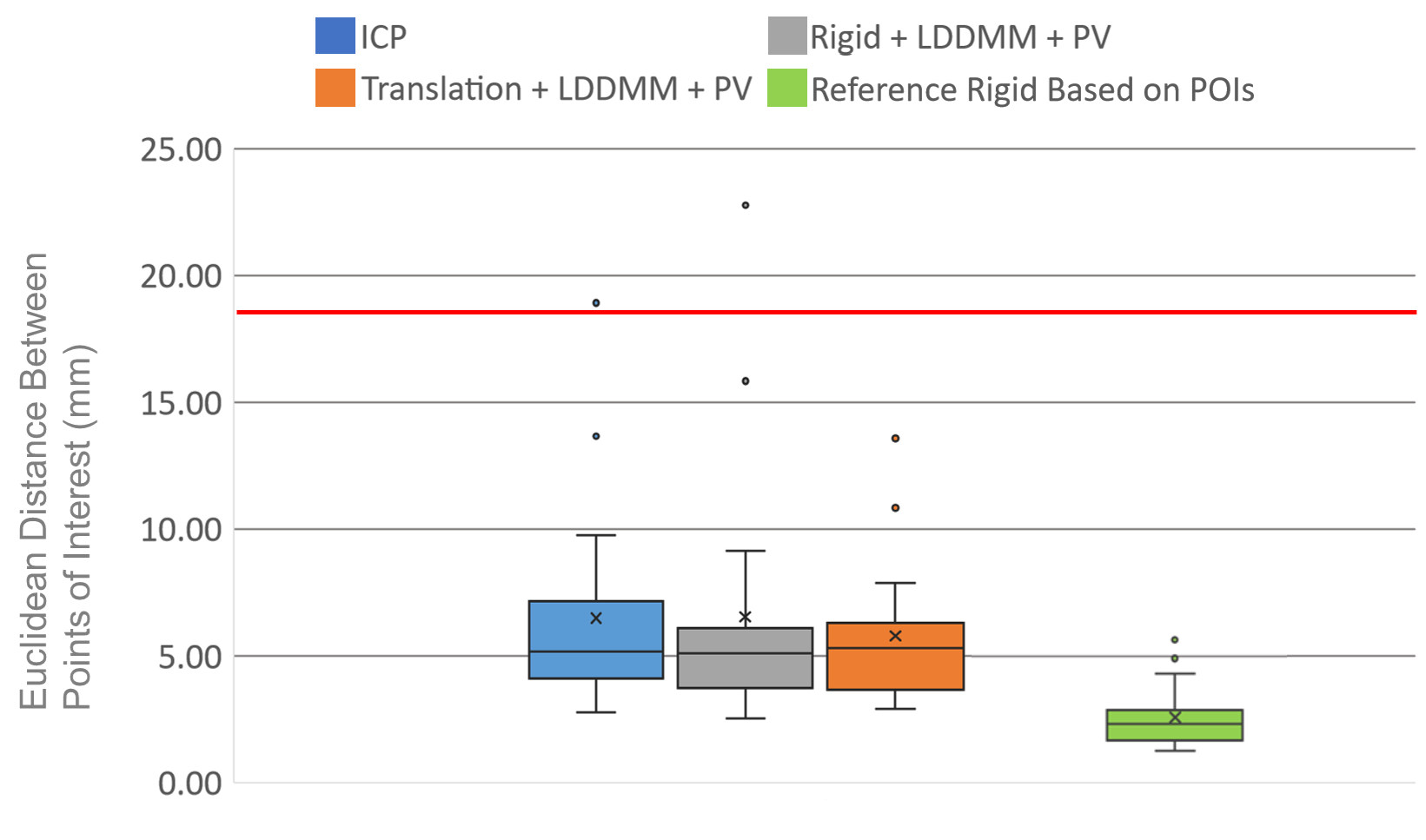
We computed the euclidean distance between the POIs in the target volumes and the deformed ones. The results are presented in two figures: the first one (Fig. 7) provides a detail of the distances between the POIs as a function of the average distances from the points of the deformed surface to those of the target surface. This gives an idea of the distance between the edges of the liver after registration and the influence on the distance between the POIs. The associated box plots in Fig. 8 provide a summary of the interest point registration results according to the method used.
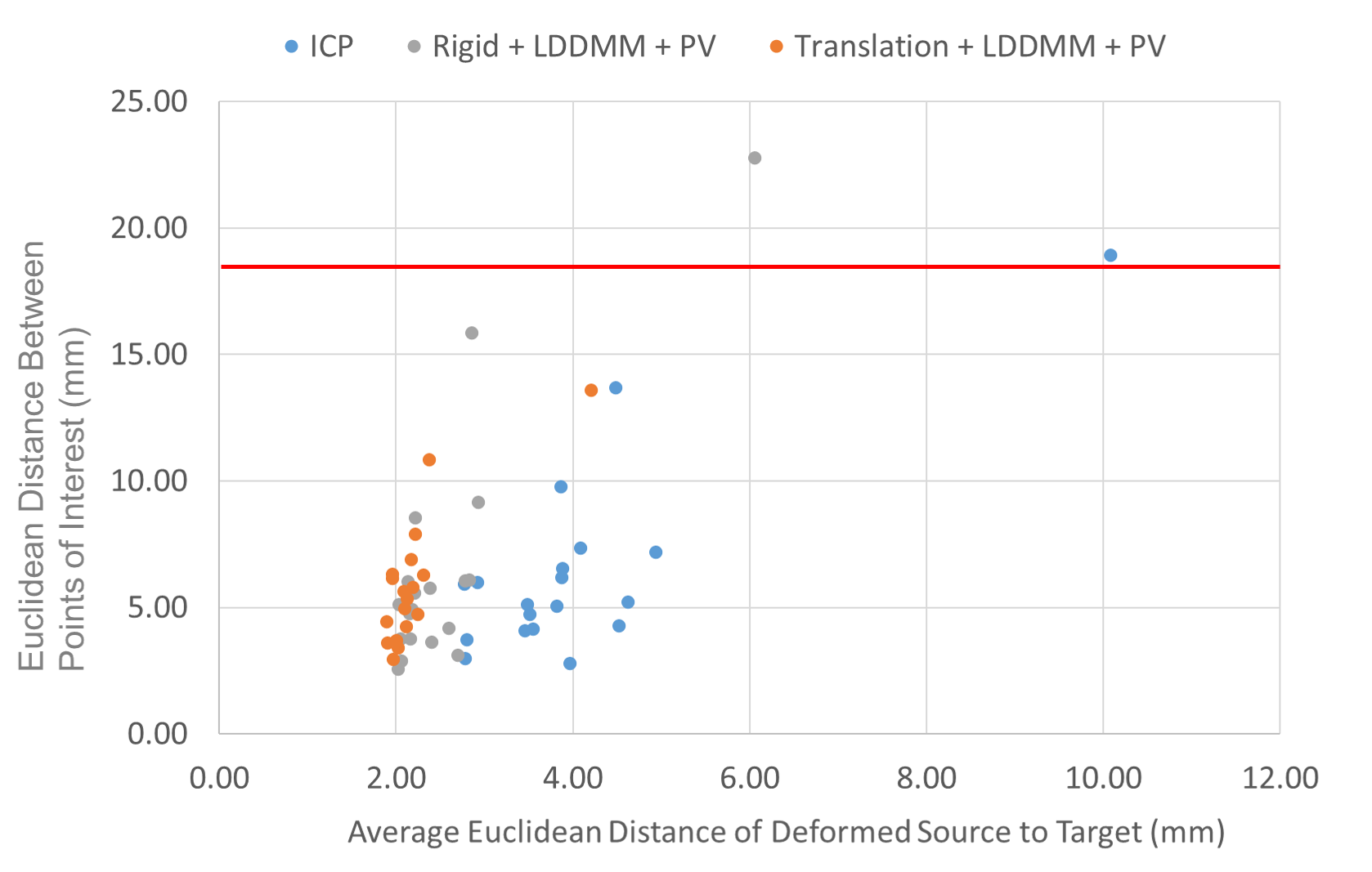
The right box in Fig. 8 corresponds to the ICP rigid registration based on the POIs for the data attachment term and is used as reference. Note that this box shows that the variations cannot be explained by rigid deformations only. We observe in Fig. 7 that the LDDMM deformations allow a consistent and robust registration of the surfaces with an average distance of the deformed source points to the target of about in average. This cannot be achieved by only rigid deformations guided by ICP ( in average), but must be validated with other metric to assess the quality of the deformation applied to the whole livers volumes. In terms of POIs distances, none of the three methods illustrated in this scatter plot shows significant difference with the others, as validated in Fig. 8.
Each of them performs differently depending on which patient they are evaluated as one can see in the detailed table in Appendix A, but none of them stands out for the POIs metric. The best average performance is achieved with the translation+LDDMM deformation guided by our partial dissimilarity term yet it is not significantly better that the rigid ICP () or the rigid+LDDMM method (). When referring to the details in Appendix A, we see that the LDDMM deformations significantly improve the translations (reducing by the distance between the POIs). However, rigid registrations provide a poor initialization for the LDDMM deformations.
By looking at the rotations angles obtained with the ICP based on the surfaces in Table 3 (Appendix C), we observe a difference with those obtained with the reference rigid registration based on the POIs. The wrong rotations of the rigid ICP based on the surfaces come from the truncation of the source which can be interpreted as less constraints for the registration problem. Similar results are observed for the rigid registration guided by the partial varifold term. In such cases, the LDDMM fails to compensate for the error that causes the non-rigid deformation to start in a local minimum. It is illustrated in Fig. 6, where the vessel and the tumor are clearly mismatched for the volumes deformed by approaches using a rigid transformation.
Inherently, we will not be able to do better than the reference method based on POIs, but we observe that the surface-based registration provides satisfactory results on the whole. When viewing the results, the points of interest are quickly found from one volume to another, even for Patient 14 which is the outlier. Even in this case (first row of Appendix D) we can see that the structures are not so far apart visually, which illustrates a certain robustness of the registrations. In particular, the partial varifold term allows both rigid and non-rigid consistent registrations with respect to the metric on the POIs.
Fig. 5 displays the results for Patient 11. This case corresponds to the best result in terms of POIs distance (), which is achieved by the rigid method guided by the ICP. Yet this case illustrates that a good alignment of the POIs does not guarantee a good alignment of the tumors: tumors boundaries have been highlighted for better visibility.
3.5.2 Evaluation on the Tumors
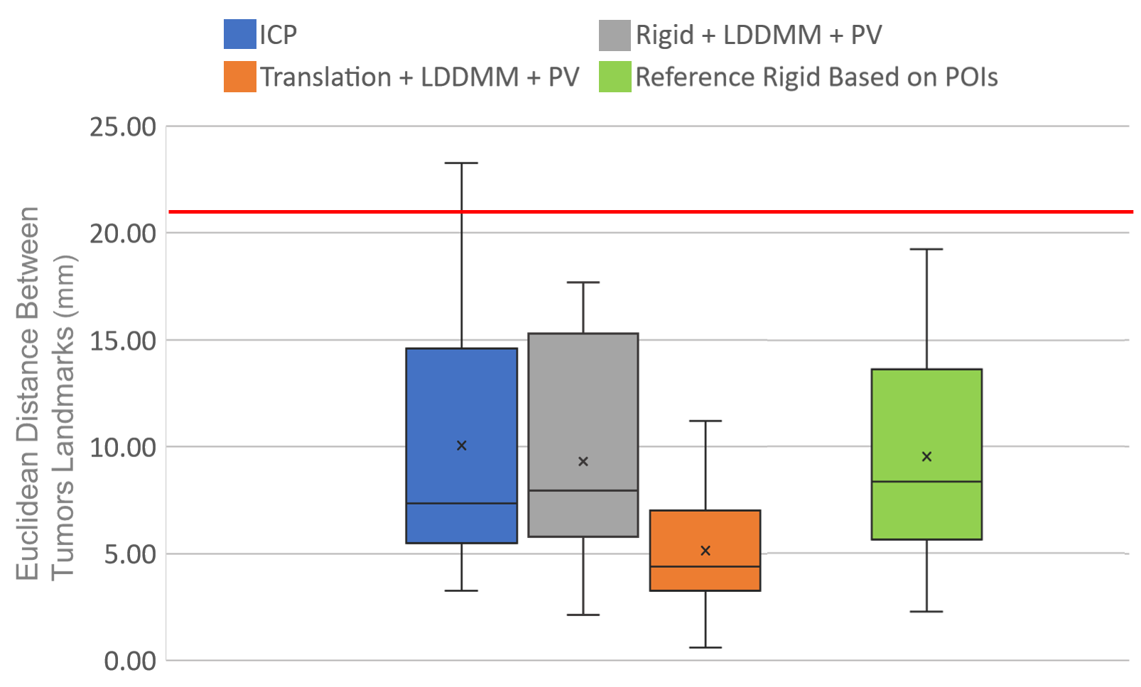
In the Figure 9 we show the metric results for the lesions landmarks that we resume per approach in Figure 10 and a detailed table is provided in Appendix B.
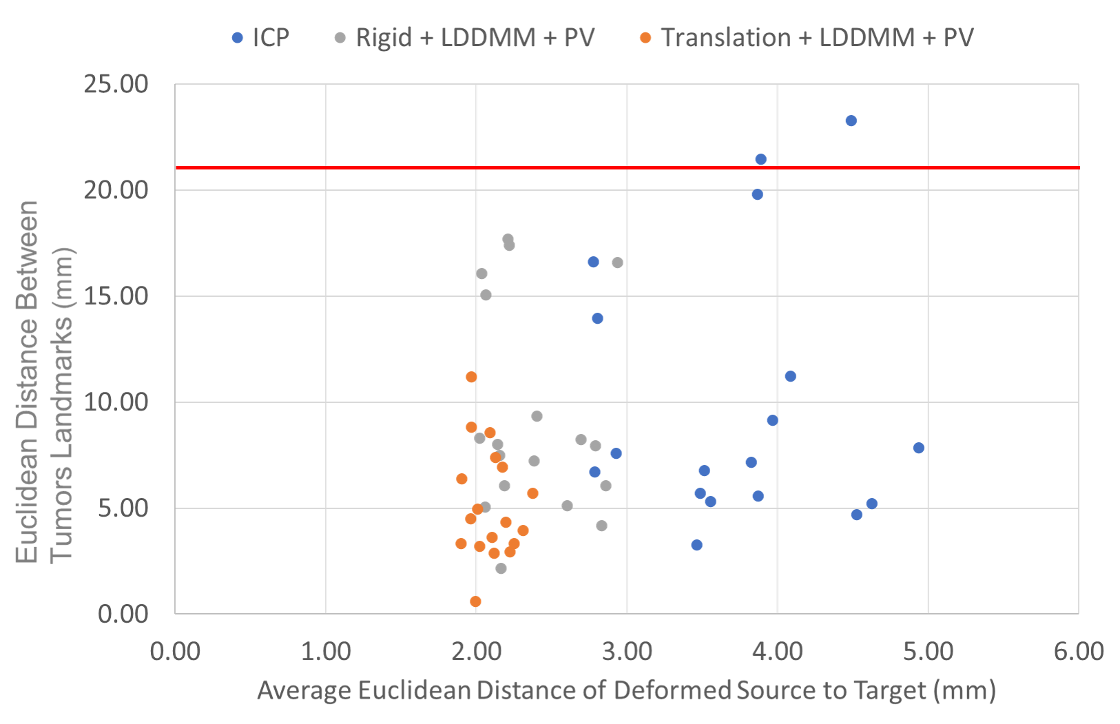
The first remarkable result is that the methods using rigid deformations fail to register the tumors closer than about in average while the translation+LDDMM guided by the partial varifold term maintains the same performance level as for the POIs metric with an average distance of . In the scatter plot of Fig. 9 we observe that the rigid ICP and the rigid+LDDMM are more spread than in the scatter plot with the metric on the POIs. In particular, the reference deformation optimized with the POIs does not perform well on the tumor registration. The main reason is that none of the POIs is located on the tumor. In fact the results of rigid ICP and rigid+LDDMM Partial Varifolds are similar to those of the reference rigid registration. These observations suggest that the rigid deformation, based on surfaces or POIs, is not always the global solution to the volume registration and may lead to local minimum. In addition, the non-rigid deformations driven by LDDMM do not improve rigid registration, despite the limitation of the rotation angles.
There is a clear difference between these methods and the registration with translation+LDDMM.
Fig. 6 (Patient 2), second row, shows a case for which the translation+LDDMM was better overall. In such case, the rotations based on the surfaces could not explain the registration between the volumes with a poor result on the lesion metric (about ). On the contrary, the translation only guided by partial matching shows performance of that is further improved by with LDDMM for a distance between the lesion landmarks of .
In Appendix D, first row, is illustrated the worst case (Patient 14) for which the infiltrated tumor was not annotated, and the liver is hardly visible in CBCT. Comparing the results of rigid+LDDMM in Appendix B and Appendix A, we see that the LDDMM deformations fail to improve significantly the rigid registration guided by the partial matching in the space of varifolds both regarding the POIs metric and the tumors one. The best initialization for the non-rigid deformations of LDDMM is the translation, providing consistent results for both metrics.
3.6 Discussion
We applied the proposed partial matching dissimilarity term to the registration of pre-op CT volumes on CBCT volumes acquired during the interventions based on segmented liver surfaces. These surfaces, truncated in CBCT, present non-rigid deformations between them due to differences in time point and patient stances in each modality. Partial matching can be used in a rigid registration process, providing results equivalent to a standard method like ICP. It is important to note that the registered surfaces in this application are relatively smooth, which favors the ICP for the rigid registration part. However, this approach in the non-rigid case can lead to projecting several points on one point of the target, and does not take into account the local orientations of the objects or their resolution. On less regular anatomies, one could expect less good performances. Moreover, this approach tends to minimize the average distance from the deformed source to the target. In some cases, as for patient 2 or patient 9, the truncation allows a freedom of deformation which makes the method unsuitable and leads to errors, whereas the reference method generating rigid deformations allowed to obtain good results on both POIs and tumor landmarks. In some cases (Patients 1, 2, 9 for instance), the reference rigid method is providing better results than the rigid ICP based on the livers surfaces, which ensures that despite an acceptable global rigid deformation, the rigid ICP fails at retrieving the correct one using the surfaces to drive the registrations.
The proposed Partial Matching can also be used in LDDMM, providing the tools of computational anatomy and allowing non-rigid, yet regular, deformations. The diffeomorphic deformations that this generates lead to accurate registration of the surfaces of the livers (about on average), which gives the physician a first tool to easily compare CT and CBCT volumes during the procedure. However, the areas of interest for the procedures are also within the liver, and care must be taken to ensure that the non-rigid deformations generated from the surfaces generalize well within the liver volume.
The distance between the Points of Interest, close to the bifurcation of the proper hepatic artery, provide a first evaluation metric to the registration methods. However, since they do not cover the volume of the livers correctly, it does not allow to discriminate between the deformation models. Regarding their location, a rigid registration is sufficient to align them when it fails to extend to the tumors landmarks as illustrated in Fig. 5. In particular, the extremities of the livers seem to be deformed by non-rigid deformations which can be explained by the better performance of the translation+LDDMM regarding the distance on the tumor landmarks. In this case, the rigid deformations with rotation lead to a local minimum that the LDDMM are unable to compensate. On the contrary, translation+LDDMM provide a consistent registration of both POIs and tumors. This last finding indicates that the correct deformations to generate to register a liver from a CBCT acquisition to the liver from the CT acquisition are translations and local non-rigid deformations without large (or even no) rotations.
Although the methods based on surface registrations are sensitive to surface extraction, we have seen through one case illustrated in Appendix D that the proposed registrations remain suitable, despite the outlier (Patient 14) with respect to the metric on the POIs. In particular natural the regularization of the LDDMM associated to the one proposed in this paper provide a smooth and consistent non rigid registration of the surface and its ambient space, ensuring realistic registrations of the volumes.
Regarding the computation time, we are studying a non-rigid multi-modality volume registration solution with partial matching. The current computation time does not allow to use this registration as is in a real time procedure, however there are many levers to accelerate the diffeomorphic deformations, main source of computation cost. These solutions, such as limiting the number of control points (and therefore variables), could allow the use of this solution in an application used during the procedures.
The purpose of this study is to provide a visualization tool for the transcatheter directed liver therapies in minimally invasive procedures. The results obtained with the translation+LDDMM method thus provide robust metrics around on average, which is useful for physicians in the perspective of navigating their tools in the patient’s anatomy to locate structures that are hardly visible in the CBCT used during the procedure. Such registrations could facilitate the physician’s intervention by providing, for example through image fusion, an improved visualization of the pre-procedure CT volume tumor placed in the CBCT volume. This would allow the physician to avoid redoing a traditional CBCT to see the tumor correctly, thus limiting the X-ray dose sent to the patient and the time of the procedure.
4 Conclusion
In this paper we adapted dissimilarity metrics in the space of varifolds to guide partial shape matching and registration. This data attachment term is suited to different shapes comparison such as unions of curves or surfaces. As a clinical application, we showed that this new partial matching term is suitable for the registration of a truncated surface onto a complete one, providing realistic feature-based CT-CBCT volumes registration. Regarding the simplicity of the shapes, the rigid ICP shows equivalent results to rigid deformations associated with the proposed partial matching. Yet this term can also be associated with a LDDMM registration and allow diffeomorphic deformations. Provided a correct feature extraction, such registrations could facilitate the physicians procedures during transcatheter directed liver therapies to treat primary and secondary liver malignancies.
In this application we only used one feature extracted from the volumes. In order to better align the CT and CBCT volumes, we could extend the feature extraction to different structures that can be observed in both modalities, such as the hepatic vascular tree, which is partially visible in the CT and in detail in the CBCT. The dissimilarity term introduced can also be modified to fit the problem of registering a complete shape onto a truncated one. The main bottleneck of our approach is the risk of shrinkage when no easy registration is possible. Apart from regularization proposed in this paper, a promising lead to tackle this issue would be to also find a subset of the target to include in the source, such as done in Bronstein et al. (2009).
Acknowledgments
This work was supported by GE Healthcare. We also would like to thank Raphael Doustaly for his technical support and discussions on the subject of multi-modality volumes registration.
Ethical Standards
The work follows appropriate ethical standards in conducting research and writing the manuscript, following all applicable laws and regulations regarding treatment of animals or human subjects.
Conflicts of Interest
We declare we don’t have conflicts of interest.
References
- Aiger et al. (2008) Dror Aiger, Niloy Mitra, and Daniel Cohen-Or. 4-points congruent sets for robust pairwise surface registration. 35th International Conference on Computer Graphics and Interactive Techniques (SIGGRAPH’08), 27, 08 2008. doi: 10.1145/1399504.1360684.
- Antonsanti et al. (2021) Pierre-Louis Antonsanti, Joan Glaunès, Thomas Benseghir, Vincent Jugnon, and Irène Kaltenmark. Partial matching in the space of varifolds. Information Processing in Medical Imaging, 2021.
- Bashiri et al. (2018) Fereshteh S. Bashiri, Ahmadreza Baghaie, Reihaneh Rostami, Zeyun Yu, and Roshan D’Souza. Multi-modal medical image registration with full or partial data: A manifold learning approach. Journal of Imaging, 5:5, 12 2018. doi: 10.3390/jimaging5010005.
- Bauer et al. (2021) Dominik Bauer, Tom Russ, Barbara Waldkirch, Christian Tönnes, William Segars, Lothar Schad, Frank Zöllner, and Alena-Kathrin Golla. Generation of annotated multimodal ground truth datasets for abdominal medical image registration. International Journal of Computer Assisted Radiology and Surgery, 16, 05 2021. doi: 10.1007/s11548-021-02372-7.
- Beg et al. (2005) Mirza Faisal Beg, Michael Miller, Alain Trouvé, and Laurent Younes. Computing large deformation metric mappings via geodesic flows of diffeomorphisms. International Journal of Computer Vision, 61:139–157, 02 2005. doi: 10.1023/B:VISI.0000043755.93987.aa.
- Bronstein et al. (2009) Alexander Bronstein, Michael Bronstein, Alfred Bruckstein, and Ron Kimmel. Partial similarity of objects, or how to compare a centaur to a horse. International Journal of Computer Vision, 84:163–183, 08 2009. doi: 10.1007/s11263-008-0147-3.
- Bronstein et al. (2006) Alexander M. Bronstein, Michael M. Bronstein, and Ron Kimmel. Generalized multidimensional scaling: A framework for isometry-invariant partial surface matching. Proceedings of the National Academy of Sciences, 103(5):1168–1172, 2006. ISSN 0027-8424. doi: 10.1073/pnas.0508601103. URL https://www.pnas.org/content/103/5/1168.
- Charlier et al. (2021) Benjamin Charlier, Jean Feydy, Joan Alexis Glaunès, François-David Collin, and Ghislain Durif. Kernel operations on the gpu, with autodiff, without memory overflows. Journal of Machine Learning Research, 22(74):1–6, 2021. URL http://jmlr.org/papers/v22/20-275.html.
- Charon and Trouvé (2013) Nicolas Charon and Alain Trouvé. The varifold representation of nonoriented shapes for diffeomorphic registration. SIAM Journal on Imaging Sciences, 6(4):2547–2580, 2013. doi: 10.1137/130918885.
- Charon et al. (2020) Nicolas Charon, Benjamin Charlier, Joan Glaunès, Pietro Gori, and Pierre Roussillon. 12 - fidelity metrics between curves and surfaces: currents, varifolds, and normal cycles. In Xavier Pennec, Stefan Sommer, and Tom Fletcher, editors, Riemannian Geometric Statistics in Medical Image Analysis, pages 441 – 477. Academic Press, 2020. ISBN 978-0-12-814725-2. doi: https://doi.org/10.1016/B978-0-12-814725-2.00021-2. URL http://www.sciencedirect.com/science/article/pii/B9780128147252000212.
- Christensen et al. (1996) G.E. Christensen, R.D. Rabbitt, and M.I. Miller. Deformable templates using large deformation kinematics. IEEE Transactions on Image Processing, 5(10):1435–1447, 1996. doi: 10.1109/83.536892.
- Feragen et al. (2015) Aasa Feragen, Jens Petersen, Marleen de Bruijne, and et al. Geodesic atlas-based labeling of anatomical trees: Application and evaluation on airways extracted from ct. IEEE Transactions on Medical Imaging, 34:1212–1226, 2015.
- Feydy et al. (2017) Jean Feydy, Benjamin Charlier, François-Xavier Vialard, and Gabriel Peyré. Optimal transport for diffeomorphic registration. Lecture Notes in Computer Science, page 291–299, 2017. ISSN 1611-3349. URL http://dx.doi.org/10.1007/978-3-319-66182-7˙34.
- Ghosn et al. (2021) Mario Ghosn, H. Derbel, R. Kharrat andN. Oubaya, S. Mulé, J. Chalaye, H. Regnault, G. Amaddeo, E. Itti, A. Luciani, H. Kobeiter, and V. Tacher. Prediction of overall survival in patients with hepatocellular carcinoma treated with y-90 radioembolization by imaging response criteria. Diagnostic and Interventional Imaging, 102:35–44, 08 2021.
- Glaunès (2005) Joan Glaunès. Transport par difféomorphismes de points, demesures et de courants pour la comparaison de formes et l’anatomie numérique.PhD thesis, Université Paris 13, 2005.
- Halimi et al. (2019) O. Halimi, O. Litany, E. R. Rodolà, A. M. Bronstein, and R. Kimmel. Unsupervised learning of dense shape correspondence. 2019 IEEE/CVF Conference on Computer Vision and Pattern Recognition (CVPR), pages 4365–4374, 2019. doi: 10.1109/CVPR.2019.00450.
- Halimi et al. (2020) Oshri Halimi, Ido Imanuel, Or Litany, Giovanni Trappolini, Emanuele Rodolà, Leonidas J. Guibas, and Ron Kimmel. The whole is greater than the sum of its nonrigid parts. CoRR, abs/2001.09650, 2020. URL https://arxiv.org/abs/2001.09650.
- Hsieh and Charon (2021) Hsi-Wei Hsieh and Nicolas Charon. Diffeomorphic registration with density changes for the analysis of imbalanced shapes. Information Processing in Medical Imaging, pages 31–42, 2021.
- Jiang et al. (2021) Xingyu Jiang, Jiayi Ma, Guobao Xiao, Zhenfeng Shao, and Xiaojie Guo. A review of multimodal image matching: Methods and applications. Information Fusion, 73:22–71, 2021. ISSN 1566-2535. doi: https://doi.org/10.1016/j.inffus.2021.02.012. URL https://www.sciencedirect.com/science/article/pii/S156625352100035X.
- Kaltenmark and Trouvé (2018) Irène Kaltenmark and Alain Trouvé. Estimation of a Growth Development with Partial Diffeomorphic Mappings. Quaterly of Applied MAthematics, 77:227–267, November 2018.
- Kaltenmark et al. (2017) Irene Kaltenmark, Benjamin Charlier, and Nicolas Charon. A general framework for curve and surface comparison and registration with oriented varifolds. Proceedings of the IEEE Conference on Computer Vision and Pattern Recognition (CVPR), July 2017.
- Miller et al. (2006) Michael I. Miller, Alain Trouvé, and Laurent Younes. Geodesic shooting for computational anatomy. Journal of Mathematical Imaging and Vision, 24(2):209–228, Mar 2006. ISSN 1573-7683.
- Milletari et al. (2016) Fausto Milletari, Nassir Navab, and Seyed-Ahmad Ahmadi. V-net: Fully convolutional neural networks for volumetric medical image segmentation. 2016 fourth international conference on 3D vision (3DV), pages 565–571, 10 2016. doi: 10.1109/3DV.2016.79.
- Mori et al. (2013) Kensaku Mori, Ichiro Sakuma, Yoshinobu Sato, Christian Barillot, and Nassir Navab, editors. Iterative Closest Curve: A Framework for Curvilinear Structure Registration Application to 2D/3D Coronary Arteries Registration, Berlin, Heidelberg, 2013. Springer Berlin Heidelberg.
- Musy et al. (2021) Marco Musy, Guillaume Jacquenot, Giovanni Dalmasso, neoglez, Ruben de Bruin, Ahinoam Pollack, Federico Claudi, Codacy Badger, icemtel, Bane Sullivan, Brian Lerner, Daniel Hrisca, Diego Volpatto, Nico Schlömer, RichardScottOZ, Zhi-Qiang Zhou, and ilorevilo. marcomusy/vedo: 2021.0.7, November 2021. URL https://doi.org/10.5281/zenodo.5655358.
- Ovsjanikov et al. (2012) Maks Ovsjanikov, Mirela Ben-Chen, Justin Solomon, Adrian Butscher, and Leonidas Guibas. Functional maps: A flexible representation of maps between shapes. ACM Trans. Graph., 31(4), July 2012. ISSN 0730-0301. doi: 10.1145/2185520.2185526.
- Paszke et al. (2017) Adam Paszke, Sam Gross, Soumith Chintala, Gregory Chanan, Edward Yang, Zachary DeVito, Zeming Lin, Alban Desmaison, Luca Antiga, and Adam Lerer. Automatic differentiation in PyTorch. In NIPS Autodiff Workshop, 2017.
- Rajagopal and Venkatesan (2016) M. Rajagopal and AM. Venkatesan. Image fusion and navigation platforms for percutaneous image-guided interventions. Abdom Radiol (NY), 41:620–628, 04 2016. doi: 10.1007/s00261-016-0645-7.
- Rodolà et al. (2017) E. Rodolà, L. Cosmo, M. M. Bronstein, A. Torsello, and D. Cremers. Partial functional correspondence. Computer Graphics Forum, 36(1):222–236, 2017. doi: https://doi.org/10.1111/cgf.12797.
- Rodolà et al. (2013) Emanuele Rodolà, Andrea Albarelli, Filippo Bergamasco, and Andrea Torsello. A scale independent selection process for 3d object recognition in cluttered scenes. International Journal of Computer Vision, 102, 03 2013. doi: 10.1007/s11263-012-0568-x.
- Sotiras et al. (2013) A. Sotiras, C. Davatzikos, and N. Paragios. Deformable medical image registration: A survey. IEEE Transactions on Medical Imaging, 32(7):1153–1190, July 2013. ISSN 1558-254X. doi: 10.1109/TMI.2013.2265603.
- Sukurdeep et al. (2021) Yashil Sukurdeep, Martin Bauer, and Nicolas Charon. A new variational model for the analysis of shape graphs with partial matching constraints. arXiv preprint arXiv:2105.00678, 2021.
- Tacher et al. (2015) V. Tacher, A. Radaelli, M. Lin, and JF. Geschwind. How i do it: Cone-beam ct during transarterial chemoembolization for liver cancer. Radiology, 274:320–334, 02 2015. doi: 10.1148/radiol.14131925.
- Trouvé (1995) Alain Trouvé. Infinite-dimensional group action and pattern-recognition. COMPTES RENDUS DE L ACADEMIE DES SCIENCES SERIE I-MATHEMATIQUE, 321(8):1031–1034, 1995.
- van Kaick et al. (2011) Oliver van Kaick, Hao Zhang, Ghassan Hamarneh, and Daniel Cohen-Or. A survey on shape correspondence. Computer Graphics Forum, 30(6):1681–1707, 2011. URL https://onlinelibrary.wiley.com/doi/abs/10.1111/j.1467-8659.2011.01884.x.
- van Kaick et al. (2013) Oliver van Kaick, Hao Zhang, and Ghassan Hamarneh. Bilateral maps for partial matching. Computer Graphics Forum (CGF), 09 2013. doi: 10.1111/cgf.12084.
- Zhao et al. (2015) Qingyu Zhao, James Price, S. Pizer, M. Niethammer, R. Alterovitz, and J. Rosenman. Surface registration in the presence of missing patches and topology change. In MIUA, 2015.
A POIs Detailed Results per Patients
| Patients | ICP Rigid | Rigid |
| Translation |
|
| ||||||
|---|---|---|---|---|---|---|---|---|---|---|---|---|
| Patient 0 | 5.18 | 4.29 | 4.15 | 18.6 | 4.71 | 2.47 | ||||||
| Patient 1 | 7.33 | 22.5 | 15.8 | 14.1 | 7.86 | 4.32 | ||||||
| Patient 2 | 9.75 | 9.88 | 8.53 | 12.8 | 4.94 | 4.92 | ||||||
| Patient 3 | 5.9 | 5.97 | 5.09 | 9.09 | 6.14 | 2.87 | ||||||
| Patient 4 | 5.04 | 5.95 | 6.05 | 8.31 | 6.89 | 5.66 | ||||||
| Patient 5 | 5.1 | 6.14 | 4.89 | 5.06 | 3.37 | 2.26 | ||||||
| Patient 6 | 4.26 | 4.42 | 6.08 | 6.91 | 10.8 | 1.28 | ||||||
| Patient 7 | 4.06 | 2.93 | 3.75 | 6.36 | 3.6 | 1.74 | ||||||
| Patient 8 | 4.72 | 3.55 | 4.76 | 5.87 | 3.67 | 2.36 | ||||||
| Patient 9 | 13.7 | 7.4 | 9.14 | 14.0 | 6.26 | 1.66 | ||||||
| Patient 10 | 3.7 | 2.93 | 2.88 | 5.25 | 2.93 | 1.65 | ||||||
| Patient 11 | 2.77 | 3.48 | 3.61 | 8.87 | 4.22 | 1.48 | ||||||
| Patient 12 | 5.97 | 5.31 | 6.02 | 9.03 | 6.3 | 3.02 | ||||||
| Patient 13 | 6.53 | 5.71 | 5.56 | 13.4 | 5.6 | 2.47 | ||||||
| Patient 14 | 18.9 | 22.3 | 22.8 | 28.1 | 13.6 | 1.69 | ||||||
| Patient 15 | 2.97 | 2.3 | 2.55 | 6.46 | 3.59 | 2.64 | ||||||
| Patient 16 | 4.12 | 3.34 | 3.75 | 4.07 | 4.4 | 2.28 | ||||||
| Patient 17 | 6.17 | 11.0 | 3.1 | 5.72 | 5.32 | 2.34 | ||||||
| Patient 18 | 7.17 | 7.05 | 5.74 | 13.9 | 5.76 | 1.89 | ||||||
| Average | 6.49 | 7.18 | 6.54 | 10.3 | 5.79 | 2.58 | ||||||
| Stdev | 3.93 | 5.83 | 4.95 | 5.9 | 2.66 | 1.18 | ||||||
| Median | 5.18 | 5.71 | 5.09 | 8.87 | 5.32 | 2.34 |
B Lesions Detailed Results per Patients
| Patients | ICP Rigid | Rigid |
| Translation |
|
| ||||||
|---|---|---|---|---|---|---|---|---|---|---|---|---|
| Patient 0 | 5.19 | 3.94 | 5.11 | 17.6 | 3.31 | 13.6 | ||||||
| Patient 1 | 11.2 | 18.2 | 6.05 | 1.41 | 2.93 | 5.2 | ||||||
| Patient 2 | 19.8 | 18.8 | 17.4 | 10.8 | 3.62 | 2.21 | ||||||
| Patient 3 | 16.6 | 16.8 | 16.0 | 16.7 | 11.2 | 14.0 | ||||||
| Patient 4 | 7.14 | 9.34 | 7.92 | 9.78 | 6.91 | 13.7 | ||||||
| Patient 5 | 5.68 | 6.77 | 6.03 | 7.25 | 3.18 | 8.0 | ||||||
| Patient 6 | 4.67 | 4.32 | 4.15 | 4.37 | 5.7 | 12.0 | ||||||
| Patient 7 | 3.24 | 4.02 | 2.14 | 2.8 | 0.59 | 6.39 | ||||||
| Patient 8 | 6.76 | 6.17 | 7.48 | 6.77 | 4.93 | 5.76 | ||||||
| Patient 9 | 23.3 | 18.4 | 16.6 | 6.86 | 3.94 | 8.68 | ||||||
| Patient 10 | 13.9 | 14.4 | 15.1 | 13.0 | 8.81 | 9.15 | ||||||
| Patient 11 | 9.12 | 7.49 | 9.32 | 3.66 | 2.86 | 18.7 | ||||||
| Patient 12 | 7.56 | 8.22 | 8.0 | 6.73 | 4.48 | 4.04 | ||||||
| Patient 13 | 21.4 | 21.2 | 17.7 | 22.7 | 8.55 | 13.4 | ||||||
| Patient 14 | None | None | None | None | None | None | ||||||
| Patient 15 | 6.69 | 7.36 | 8.28 | 9.49 | 6.36 | 19.3 | ||||||
| Patient 16 | 5.31 | 4.7 | 5.03 | 6.96 | 3.3 | 6.97 | ||||||
| Patient 17 | 5.56 | 12.5 | 8.22 | 7.29 | 7.37 | 2.87 | ||||||
| Patient 18 | 7.83 | 7.75 | 7.21 | 12.0 | 4.32 | 7.44 | ||||||
| Average | 10.1 | 10.6 | 9.31 | 9.23 | 5.13 | 9.52 | ||||||
| StDev | 6.06 | 5.71 | 4.8 | 5.37 | 2.56 | 5.08 | ||||||
| Median | 7.35 | 7.98 | 7.96 | 7.27 | 4.4 | 8.34 |
C Rotations Deformations Comparison
| Rigid ICP Based POIs | Rigid ICP Based Surfaces | |||||
|---|---|---|---|---|---|---|
| Patients | X | Y | Z | X | Y | Z |
| Patient 0 | -1.15 | -11.52 | 14.2 | -1.53 | -12.18 | 10.7 |
| Patient 1 | -5.58 | -11.68 | 0.8 | -9.69 | -6.51 | 3.89 |
| Patient 2 | -8.66 | -6.28 | -0.03 | -17.39 | -2.59 | 0.64 |
| Patient 3 | -13.49 | -0.11 | 2.58 | -13.03 | 0.51 | 1.33 |
| Patient 4 | -9.02 | 3.17 | -10.8 | -8.37 | 0.93 | -9.45 |
| Patient 5 | -2.37 | -4.13 | -2.43 | -4.96 | -1.93 | 1.89 |
| Patient 6 | -5.09 | -1.27 | -3.64 | -6.42 | 0.65 | -4.96 |
| Patient 7 | -6.13 | 2.37 | -5.04 | -4.85 | 0.85 | -3.43 |
| Patient 8 | -6.36 | 4.98 | 6.14 | -6.81 | 3.45 | 2.47 |
| Patient 9 | -0.77 | -5.45 | 8.57 | -3.49 | -12.56 | 6.15 |
| Patient 10 | 2.49 | 6.94 | 3.18 | -0.72 | 6.71 | 3.68 |
| Patient 11 | -10.15 | -5.21 | 1.52 | -9.34 | -3.62 | 0.27 |
| Patient 12 | 5.1 | 4.96 | -6.6 | 5.3 | 4.18 | -4.14 |
| Patient 13 | -5.25 | -2.79 | 11.2 | -2.5 | -6.93 | 10.2 |
| Patient 14 | 3.3 | -12.94 | -4.14 | -9.25 | -16.26 | 6.0 |
| Patient 15 | -2.38 | 6.39 | -5.4 | -3.88 | 6.68 | -5.35 |
| Patient 16 | 1.71 | -1.56 | 1.45 | -2.71 | -2.01 | 0.31 |
| Patient 17 | -0.93 | -1.01 | 4.24 | -4.11 | -2.33 | 7.57 |
| Patient 18 | -3.28 | 10.3 | -4.61 | 4.76 | 9.8 | 0.54 |
D Worst Case Scenario : Bad Feature Extraction
Rigid
Rigid+LDDMM
Translation+LDDMM
with ICP
with Partial Varifold
with Partial Varifold
Surface metric : 10.1mm
Surface metric : 6.06mm
Surface metric : 4.22mm