Distributionally Robust Deep Learning using Hardness Weighted Sampling
Lucas Fidon1, Michael Aertsen2, Thomas Deprest2, Doaa Emam3, Frédéric Guffens2, Nada Mufti4, Esther Van Elslander2, Ernst Schwartz5, Michael Ebner4, Daniela Prayer5, Gregor Kasprian5, Anna L David6, Andrew Melbourne4, Sébastien Ourselin4, Jan Deprest3, Georg Langs5, Tom Vercauteren4
1: Shool of Biomedical Engineering & Imaging Sciences, King's College London, 2: Department of Radiology, University Hospitals Leuven, 3: Department of Obstetrics and Gynaecology, University Hospitals Leuven, 4: School of Biomedical Engineering & Imaging Sciences, King’s College London, 5: Department of Biomedical Imaging and Image-guided Therapy, Medical University of Vienna, 6: Institute for Women’s Health, University College London
Limiting failures of machine learning systems is of paramount importance for safety-critical applications. In order to improve the robustness of machine learning systems, Distributionally Robust Optimization (DRO) has been proposed as a generalization of Empirical Risk Minimization (ERM). However, its use in deep learning has been severely restricted due to the relative inefficiency of the optimizers available for DRO in comparison to the wide-spread variants of Stochastic Gradient Descent (SGD) optimizers for ERM. We propose SGD with hardness weighted sampling, a principled and efficient optimization method for DRO in machine learning that is particularly suited in the context of deep learning. Similar to a hard example mining strategy in practice, the proposed algorithm is straightforward to implement and computationally as efficient as SGD-based optimizers used for deep learning, requiring minimal overhead computation. In contrast to typical ad hoc hard mining approaches, we prove the convergence of our DRO algorithm for over-parameterized deep learning networks with ReLU activation and finite number of layers and parameters. Our experiments on fetal brain 3D MRI segmentation and brain tumor segmentation in MRI demonstrate the feasibility and the usefulness of our approach. Using our hardness weighted sampling for training a state-of-the-art deep learning pipeline leads to improved robustness to anatomical variabilities in automatic fetal brain 3D MRI segmentation using deep learning and to improved robustness to the image protocol variations in brain tumor segmentation.a decrease of 2% of the interquartile range of the Dice scores for the enhanced tumor and the tumor core regions. Our code is available at https://github.com/LucasFidon/HardnessWeightedSampler
Bibtex @article{melba:2022:019:fidon,
title = "Distributionally Robust Deep Learning using Hardness Weighted Sampling",
author = "Fidon, Lucas and Aertsen, Michael and Deprest, Thomas and Emam, Doaa and Guffens, Frédéric and Mufti, Nada and Van Elslander, Esther and Schwartz, Ernst and Ebner, Michael and Prayer, Daniela and Kasprian, Gregor and David, Anna L and Melbourne, Andrew and Ourselin, Sébastien and Deprest, Jan and Langs, Georg and Vercauteren, Tom",
journal = "Machine Learning for Biomedical Imaging",
volume = "1",
issue = "PIPPI 2021 special issue",
year = "2022",
pages = "1--61",
issn = "2766-905X",
doi = "https://doi.org/10.59275/j.melba.2022-8b6a",
url = "https://melba-journal.org/2022:019"
}
RISTY - JOUR
AU - Fidon, Lucas
AU - Aertsen, Michael
AU - Deprest, Thomas
AU - Emam, Doaa
AU - Guffens, Frédéric
AU - Mufti, Nada
AU - Van Elslander, Esther
AU - Schwartz, Ernst
AU - Ebner, Michael
AU - Prayer, Daniela
AU - Kasprian, Gregor
AU - David, Anna L
AU - Melbourne, Andrew
AU - Ourselin, Sébastien
AU - Deprest, Jan
AU - Langs, Georg
AU - Vercauteren, Tom
PY - 2022
TI - Distributionally Robust Deep Learning using Hardness Weighted Sampling
T2 - Machine Learning for Biomedical Imaging
VL - 1
IS - PIPPI 2021 special issue
SP - 1
EP - 61
SN - 2766-905X
DO - https://doi.org/10.59275/j.melba.2022-8b6a
UR - https://melba-journal.org/2022:019
ER -
Disclaimer: the following html version has been automatically generated and the PDF remains the reference version. Feedback can be sent directly to publishing-editor@melba-journal.org
1 Introduction
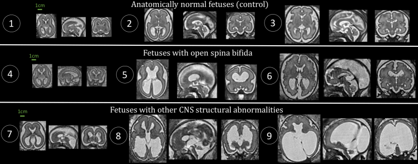
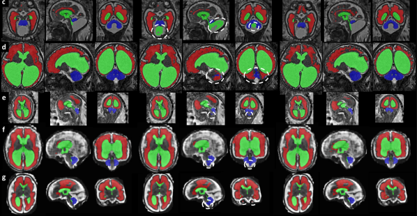
Datasets used to train deep neural networks typically contain some underrepresented subsets of cases. These cases are not specifically dealt with by the training algorithms currently used for deep neural networks. This problem has been referred to as hidden stratification (Oakden-Rayner et al., 2020). Hidden stratification has been shown to lead to deep learning models with good average performance but poor performance on underrepresented but clinically relevant subsets of the population (Larrazabal et al., 2020; Oakden-Rayner et al., 2020; Puyol-Antón et al., 2021). In Figure 1 we give an example of hidden stratification in fetal brain MRI. The presence of abnormalities associated with diseases with low prevalence (Aertsen et al., 2019) exacerbates the anatomical variability of the fetal brain between 18 weeks and 38 weeks of gestation.
While uncovering the issue, the study of Oakden-Rayner et al. (2020) does not study the cause or propose a method to mitigate this problem. In addition, the work of Oakden-Rayner et al. (2020) is limited to classification. In standard deep learning pipelines, this hidden stratification is ignored and the model is trained to minimize the mean per-example loss, which corresponds to the standard Empirical Risk Minimization (ERM) problem. As a result, models trained with ERM are more likely to underperform on those examples from the underrepresented subdomains, seen as hard examples. This may lead to unfair AI systems (Larrazabal et al., 2020; Puyol-Antón et al., 2021). For example, state-of-the-art deep learning models for brain tumor segmentation (currently trained using ERM) underperform for cases with confounding effects, such as low grade gliomas, despite achieving good average and median performance (Bakas et al., 2018). For safety-critical systems, such as those used in healthcare, this greatly limits their usage as ethics guidelines of regulators such as European Commission (2019) require AI systems to be technically robust and fair prior to their deployment in hospitals.
Distributionally Robust Optimization (DRO) is a robust generalization of ERM that has been introduced in convex machine learning to model the uncertainty in the training data distribution (Chouzenoux et al., 2019; Duchi et al., 2016; Namkoong and Duchi, 2016; Rafique et al., 2018). Instead of minimizing the mean per-example loss on the training dataset, DRO seeks to optimize for the hardest weighted empirical training data distribution around the (uniform) empirical training data distribution. This suggests a link between DRO and Hard Example Mining. However, DRO as a generalization of ERM for machine learning still lacks optimization methods that are principled and computationally as efficient as SGD in the non-convex setting of deep learning. Previously proposed principled optimization methods for DRO consist in alternating between approximate maximization and minimization steps (Jin et al., 2019; Lin et al., 2019; Rafique et al., 2018). However, they differ from SGD methods for ERM by the introduction of additional hyperparameters for the optimizer such as a second learning rate and a ratio between the number of minimization and maximization steps. This makes DRO difficult to use as a drop-in replacement for ERM in practice.
In contrast, efficient weighted sampling methods, including Hard Example Mining (Chang et al., 2017; Loshchilov and Hutter, 2016; Shrivastava et al., 2016) and weighted sampling (Berger et al., 2018; Puyol-Antón et al., 2021), have been empirically shown to mitigate class imbalance issues and to improve deep embedding learning (Harwood et al., 2017; Suh et al., 2019; Wu et al., 2017). However, even though these works typically start from an ERM formulation, it is not clear how those heuristics formally relate to ERM in theory. This suggests that bridging the gap between DRO and weighted sampling methods could lead to a principled Hard Example Mining approach, or conversely to more efficient optimization methods for DRO in deep learning.
Given an efficient solver for the inner maximization problem in DRO, DRO could be addressed by maintaining a solution of the inner maximization problem and using a minimization scheme akin to the standard ERM but over an adaptively weighted empirical distribution. However, even in the case where a closed-form solution is available for the inner maximization problem, it would require performing a forward pass over the entire training dataset at each iteration. This cannot be done efficiently for large datasets. This suggests identifying an approximate, but practically usable, solution for the inner maximization problem based on a closed-form solution.
From a theoretical perspective, analysis of previous optimization methods for non-convex DRO (Jin et al., 2019; Lin et al., 2019; Rafique et al., 2018) made the assumption that the model is either smooth or weakly-convex, but none of those properties are true for deep neural networks with activation functions that are typically used.
In this work, we propose SGD with hardness weighted sampling, a novel, principled optimization method for training deep neural networks with DRO and inspired by Hard Example Mining, that is computationally as efficient as SGD for ERM. Compared to SGD, our method only requires introducing an additional layer and maintaining a stale per-example loss vector to compute sampling probabilities over the training data. This work is an extension of our previous preliminary work (Fidon et al., 2021b) in which we applied the proposed hardnes weighted sampler to distributionally robust fetal brain 3D MRI segmentation and studied the link between DRO and the minimization of percentiles of the per-example loss. In this extension, we formally introduce our hardness weighted sampler and we generalize recent results in the convergence theory of SGD with ERM and over-parameterized deep learning networks with activation functions (Allen-Zhu et al., 2019b, a; Cao and Gu, 2020; Zou and Gu, 2019) to our SGD with hardness weighted sampling for DRO. This is, to the best of our knowledge, the first convergence result for deep learning networks with trained with DRO. We also formally link DRO in our method with Hard Example Mining. As a result, our method can be seen as a principled Hard Example Mining approach. In terms of experiments, we have extended the evaluation on fetal brain 3D MRI with additional fetal brain 3D MRIs. We have also added experiments on brain tumor segmentations and experiments on image classification with MNIST as a toy example. We show that our method outperforms plain SGD in the case of class imbalance, and improves the robustness of a state-of-the-art deep learning pipeline for fetal brain segentation and brain tumor segmentation. We evaluate the proposed methodology for the automatic segmentation of white matter, ventricles, and cerebellum based on fetal brain 3D T2w MRI. We used a total of fetal brain 3D MRIs including anatomically normal fetuses, fetuses with spina bifida aperta, and fetuses with other central nervous system pathologies for gestational ages ranging from weeks to weeks. Our empirical results suggest that the proposed training method based on distributionally robust optimization leads to better percentiles values for abnormal fetuses. In addition, qualitative results shows that distributionally robust optimization allows to reduce the number of clinically relevant failures of nnU-Net. For brain tumor segmentation our DRO-based method allows reducing the interquartile range of the Dice scores of for the segmentation of the enhancing tumor and the tumor core regions.
1.1 Main Mathematical Notations
We summarize here the main mathematical notations. An extended list of notations can be found in Appendix A.
•
Training dataset: .
•
is a -simplex.
•
Let , and a function, we denote .
•
Let , and a function, we denote .
•
is the uniform training data distribution, i.e. .
•
is the per-example loss function.
•
ERM is short for Empirical Risk Minimization.
•
DRO is short for Distributionally Robust Optimisation.
Figure 1: Illustration of the anatomical variability in fetal brain across gestational ages and diagnostics. 1: Control (22 weeks); 2: Control (26 weeks); 3: Control (29 weeks); 4: Spina bifida (19 weeks); 5: Spina bifida (26 weeks); 6: Spina bifida (32 weeks); 7: Dandy-walker malformation with corpus callosum abnormality (23 weeks); 8: Dandy-walker malformation with ventriculomegaly and periventricular nodular heterotopia (27 weeks); 9: Aqueductal stenosis (34 weeks).
2 Related Works
An optimization method for group-DRO was proposed in (Sagawa et al., 2020). In contrast to the formulation of DRO that we study in this paper, their method requires additional labels allowing to identify the underrepresented group in the training dataset. However, those labels may not be available or may even be impossible to obtain in most applications. Sagawa et al. (2020) show that, when associated with strong regularization of the weights of the network, their group DRO method can tackle spurious correlations that are known a priori in some classification problems. It is worth noting that, in contrast, no regularization was necessary in our experiments with MNIST.
Biases of convolutional neural networks applied to medical image classification and segmentation has been studied in the literature. State-of-the-art deep neural networks for brain tumor segmentation underperform for cases with confounding effects, such as low grade gliomas (Bakas et al., 2018). It has been shown that scans coming from different studies can be re-assigned with accuracy to their source using a random forest classifier (Wachinger et al., 2019). A state-of-the-art deep neural networks for the diagnosis of thoracic diseases using X-ray trained on a dataset with a gender bias underperform on X-ray of female patients (Larrazabal et al., 2020). And a state-of-the-art deep learning pipeline for cardiac MRI segmentation was found to underperform when evaluated on racial groups that were underrepresented in the training dataset (Puyol-Antón et al., 2021). To mitigate this problem, Puyol-Antón et al. (2021) proposed to use a stratified batch sampling approach during training that shares similarities with the group-DRO approach mentioned above (Sagawa et al., 2020). In contrast to our hardness weighted sampler, their stratified batch sampling approach requires additional labels, such as the racial group, that may not be available for training data. In addition, they do not study the formal relationship between the use of their stratified batch sampling approach and the training optimization problem.
In this work, we focus on DRO with a -divergence (Csiszár et al., 2004). In this case, the data distributions that are considered in the DRO problem (3) are restricted to sharing the support of the empirical training distribution. In other words, the weights assigned to the training data can change, but the training data itself remains unchanged. Another popular formulation is DRO with a Wasserstein distance (Chouzenoux et al., 2019; Duchi et al., 2016; Sinha et al., 2018; Staib and Jegelka, 2017). In contrast to -divergences, using a Wasserstein distance in DRO seeks to apply small data augmentation to the training data to make the deep learning model robust to small deformation of the data, but the sampling weights of the training data distribution typically remains unchanged. In this sense, DRO with a -divergence and DRO with a Wasserstein distance can be considered as orthogonal endeavours. While we show that DRO with -divergence can be seen as a principled Hard Exemple Mining method, it has been shown that DRO with a Wasserstein distance can be seen as a principled adversarial training method (Sinha et al., 2018; Staib and Jegelka, 2017).
The effect of multiplicative weighting during training, rather than weighted sampling used in our algorithm, has been studied empirically by (Byrd and Lipton, 2019) for image classification. They find that the effect of multiplicative weighting vanishes over training for classification tasks in which we can achieve zero loss on the training dataset. However, multiplicative weighting and weighted sampling affect the optimization dynamic in different ways. This may explain why we did not observe this vanishing effect in our experiments on classification and segmentation. Previous work have also studied empirical and convergence results of DRO for linear models (Hu and et al, 2018).
3 Methods
3.1 Background: Deep Learning with Distributionally Robust Optimization
Standard training procedures in machine learning are based on Empirical Risk Minimization (ERM) (Bottou et al., 2018). For a neural network with parameters , a per-example loss function , and a training dataset , where are the inputs and are the labels, the ERM problem corresponds to
(1)
where is the empirical uniform distribution on the training dataset and is the expected value operator as defined in section 1.1. When data augmentation is used, the number of samples can become infinite. For our theoretical results, we suppose that contains a finite number of examples. The extension of our Algorithm 1 to an infinite number of data augmentations using importance sampling is presented in section 3.2.2. Optionally, can contain a parameter regularization term that is only a function of .
The ERM training formulation assumes that is an unbiased approximation of the true data distribution. However, this is generally impossible in domains such as medical image computing. This makes models trained with ERM at risk of underperforming on images from parts of the data distribution that are underrepresented in the training dataset.
In contrast, Distributionally Robust Optimization (DRO) is a family of generalization of ERM in which the uncertainty in the training data distribution is modelled by minimizing the worst-case expected loss over an uncertainty set of training data distributions (Rahimian and Mehrotra, 2019).
In this paper, we consider training deep neural networks with DRO based on a -divergence. We denote the set of empirical training data probabilities vectors under consideration (i.e. the uncertainty set). The different probabilities vectors in correspond to all the possible weighting of the training dataset. Every in gives a weight to each training example but keep the examples the same. We use the following definition of -divergence in the remainder of the paper.
Definition 1 (Strong Convexity)
Let be differentiable on , a convex subset of and be the first derivative of . Let , is -strongly convex if for all .
Definition 2 (-divergence)
Let be two times continuously differentiable on , -strongly convex on with , and satisfying . The -divergence is defined as, for all ,
(2)
We refer to our example 1 on page 1 to highlight that the KL divergence is indeed a -divergence.
The DRO problem for which we propose an optimizer for training deep neural networks can be formally defined as
(3)
where is the uniform empirical distribution, and an hyperparameter. The choice of and controls how the unknown training data distribution is allowed to differ from . Here and thereafter, we use the notation to refer to the vector of loss values of the training samples for the value of the parameters of the neural network . In the remainder of the paper, we will refer to as the distributionally robust loss.
Our analysis of the properties of in the next sections relies on the Fenchel duality (Moreau, 1965) and the notion of Fenchel conjugate (Fenchel, 1949).
Definition 3 (Fenchel Conjugate Function)
Let be a proper function. The Fenchel conjugate of is defined as where is the inner product.
3.2 Hardness Weighted Sampling for Distributionally Robust Deep Learning
In the case where is a non-convex predictor (such as a deep neural network), existing optimization methods for the DRO problem (3) alternate between approximate minimization and maximization steps (Jin et al., 2019; Lin et al., 2019; Rafique et al., 2018), requiring the introduction of additional hyperparameters compared to SGD. However, these are difficult to tune in practice and convergence has not been proven for non-smooth deep neural networks such as those with activation functions.
In this section, we present an SGD-like optimization method for training a deep learning model with the DRO problem (3). We first highlight, in Section 3.2.1, mathematical properties that allow us to link DRO with stochastic gradient descent (SGD) combined with an adaptive sampling that we refer to as hardness weighted sampling. In Section 3.2.2, we present our Algorithm 1 for distributionally robust deep learning. Then, in Section 3.3, we present theoretical convergence results for our hardness weighted sampling.
3.2.1 A sampling approach to Distributionally Robust Optimization
The goal of this subsection is to show that a stochastic approximation of the gradient of the distributionally robust loss can be obtained by using a weighted sampler. This result is a first step towards our Algorithm 1 for efficient training with the distributionally robust loss presented in the next subsection.
To reformulate as an unconstrained optimization problem over (rather than constraining it to the -simplex ), we define
(4)
where is the characteristic function of the to the -simplex which is a closed convex set, i.e.
(5)
The distributionally robust loss in (3) can now be rewritten using the Fenchel conjugate function of . This allows us to obtain regularity properties for .
Lemma 4 (Regularity of )
If satisfies Definition 2 (i.e. can be used for a -divergence), then and satisfy the following:
(6)
(7)
(8)
Equation (7) follows from Definition 3. Proofs of (6) and (8) can be found in Appendix E. According to (6), the optimization problem (7) is strictly convex and admits a unique solution in , which we denote as
(9)
Thanks to those properties, we can now show the following lemma that is essential for the theoretical foundation of our Algorithm 1. Equation (10) states that the gradient of the distributionally robust loss is a weighted sum of the the gradients of the per-example losses (i.e. the gradients computed by the backpropagation algorithm in deep learning) with the weights given by the empirical distribution . We further show that straightforward analytical formulas exist for , and give an example of such probability distribution for the Kullback-Leibler (KL) divergence.
Lemma 5 (Stochastic Gradient of the Distributionally Robust Loss)
For all , we have
(10)
The proof is found in Appendix F. We now provide a closed-form formula for given for the KL divergence as the choice of -divergence.
Example 1
For , is the Kullback-Leibler (KL) divergence:
(11)
In this case, we have (see Appendix D for a proof)
(12)
3.2.2 Proposed Efficient Algorithm for Distributionally Robust Deep Learning
We now describe our algorithm for training deep neural networks with DRO using our hardness weighted sampling.
Algorithm 1 Training procedure for DRO with Hardness Weighted Sampling. Additional operations as compared to standard training algorithms are highlighted inblue.
1:: training dataset with the number of training samples.
2:: batch size.
3:: (any) smooth per-example loss function (e.g. cross entropy loss, Dice loss).
4:: robustness parameter defining the distributionally robust optimization problem.
5:: initial parameter vector for the model to train.
6:: initial stale per-example loss values vector.
7:initialize the time step
8:initialize the vector of stale loss values
9:while has not converged do
10: online estimation of the hardness weights
11: hardness weighted sampling
12:if importance sampling is not used then
13:
14:else
15: importance sampling weights
16: clip the weights for stability
17: update the vector of stale loss values
18:
19:SGD step or any other optimizer (e.g. SGD momentum, Adam)
20:Output:
Equation (10) implies that is an unbiased estimator of the gradient of the distributionally robust loss gradient when is sampled with respect to . This suggests that the distributionally robust loss can be minimized efficiently by SGD by sampling mini-batches with respect to at each iteration. However, even though closed-form formulas were provided in Example 1 for , evaluating exactly , i.e. doing one forward pass on the whole training dataset at each iteration, is computationally prohibitive for large training datasets.
In practice, we propose to use a stale version of the vector of per-example loss values by maintaining an online history of the loss values of the examples seen during training , where for all , is the last iteration at which the per-example loss of example has been computed. Using the Kullback-Leibler divergence as -divergence, this leads to the SGD with hardness weighted sampling algorithm proposed in Algorithm 1.
When data augmentation is used, an infinite number of training examples is virtually available. In this case, we keep one stale loss value per example irrespective of any augmentation as an approximation of the loss for this example under any augmentation.
Importance sampling is often used when sampling with respect to a desired distribution cannot be done exactly (Kahn and Marshall, 1953). In Algorithm 1, an up-to-date estimation of the per-example losses (or equivalently the hardness weights) in a batch is only available after sampling and evaluation through the network. Importance sampling can be used to compensate for the difference between the initial and the updated stale losses within this batch. We propose to use importance sampling in steps 9-10 of Algorithm 1 and highlight that this is especially useful to deal with data augmentation. Indeed, in this case, the stale losses for the examples in the batch are expected to be less accurate as they were estimated under a different augmentation. For efficiency, we use the following approximation where we have neglected the typically small change in the denominator of the . More details are given in Appendix C. To tackle the typical instabilities that can arise when using importance sampling (Owen and Zhou, 2000), the importance weights are clipped.
Compared to standard SGD-based training optimizers for the mean loss, our algorithm requires only an additional operation per iteration and to store an additional vector of scalars of size (number of training examples), thereby making it well suited for deep learning applications. The computational time and memory overheads are studied in section 4.3.
For the convergence theorem, the stopping criteria is . However, in our experiments, a fixed number of iterations is used as implemented in the state-of-the-art method nnU-Net Isensee et al. (2021).
3.3 Overview of Theoretical Results
In this section, we present convergence guarantees for Algorithm 1 in the framework of over-parameterized deep learning. We further demonstrate properties of our hardness weighted sampling that allow to clarify its link with Hard Example Mining and with the minimization of percentiles of the per-sample loss on the training data distribution.
3.3.1 Convergence of SGD with Hardness Weighted Sampling for Over-parameterized Deep Neural Networks with
Convergence results for over-parameterized deep learning have recently been proposed in (Allen-Zhu et al., 2019a). Their work gives convergence guarantees for deep neural networks with any activation functions (including ), and with any (finite) number of layers and parameters , under the assumption that is large enough. In our work, we extend the convergence theory developed by (Allen-Zhu et al., 2019a) for ERM and SGD to DRO using the proposed SGD with hardness weighted sampling and stale per-example loss vector (as stated in Algorithm 1). The proof in Appendix I.4 deals with the challenges raised by the non-linearity of with respect to the per-sample stale loss and the non-uniform dynamic sampling used in Algorithm 1.
Theorem 6 (Convergence of Algorithm 1 for neural networks with )
Let be a smooth per-example loss function, be the batch size, and . If the number of parameters is large enough, and the learning rate is small enough, then, with high probability over the randomness of the initialization and the mini-batches, Algorithm 1 (without importance sampling) guarantees after a finite number of iterations.
A detailed description of the assumption for this theorem is described in Appendix 12 and its proof can be found in Appendix I.4. Our proof does not cover the case where importance sampling is used. However, our empirical results suggest that convergence guarantees still hold with importance sampling.
3.3.2 Link between Hardness Weighted Sampling and Hard Example Mining
In this section, we discuss the relationship between the proposed hardness weighted sampling for DRO and Hard Example Mining. The following result shows that using the proposed hardness weighted sampler the hard training examples, those training examples with relatively high values of the loss, are sampled with higher probability.
Theorem 7
Let a -divergence that satisfies Definition 2, and a vector of loss values for the examples . The proposed hardness weighted sampling probabilities vector defined as in (9) verifies:
1.
For all , is an increasing function of .
2.
For all , is an non-increasing function of any for .
See Appendix G for the proof. The second part of Theorem 7 implies that as the loss of an example diminishes, the sampling probabilities of all the other examples increase. As a result, the proposed SGD with hardness weighted sampling balances exploitation (i.e. sampling the identified hard examples) and exploration (i.e. sampling any example to keep the record of hard examples up to date). Heuristics to enforce this trade-off are often used in Hard Example Mining methods (Berger et al., 2018; Harwood et al., 2017; Wu et al., 2017).
3.3.3 Link between DRO and the Minimization of a Loss Percentile
In this section, we show that the DRO problem (3) using the KL divergence is equivalent to a relaxation of the minimization of the per-example loss percentile shown thereafter in equation (13).
Instead of the average per-example loss (1), for robustness, one might be more interested in minimizing the percentile at (e.g. 5%) of the per-example loss function. Formally, this corresponds to the minimization problem
(13)
where is the empirical distribution defined by the training dataset. In other words, if , the optimal of (13) for a given value set of parameters is the value of the loss such that the per-example loss function is worse than of the time. As a result, training the deep neural network using (13) corresponds to minimizing the percentile of the per-example loss function .
Unfortunately, the minimization problem (13) cannot be solved directly using stochastic gradient descent to train a deep neural network. We now propose a tractable upper bound for and show that it can be solved in practice using distributionally robust optimization.
The Chernoff bound (Chernoff et al., 1952) applied to the per-example loss function and the empirical training data distribution states that for all and
(14)
To link this inequality to the minimization problem (13), we set and
(15)
In this case, we have
(16)
is therefore an upper bound for the optimal in equation (13), independently to the value of . Equation (13) can therefore be relaxed by
(17)
where is a hyperparameter, and where the term was dropped as being independent of . While in (17), does not appear in the optimization problem directly anymore, essentially acts as a substitute for . The higher the value of , the higher weights the per-example losses with a high value will have in (17).
We give a proof in Appendix H that (17) is equivalent to solving the following DRO problem
(18)
This is a special case of the DRO problem (3) where is chosen as the KL-divergence and it corresponds to the setting of Algorithm 1.
4 Experiments
In this section, we experiments with the proposed hardness weighted sampler for DRO as implemented in the proposed Algorithm 1. In the subsection 4.1, we give a toy example with the task of automatic classification of digits in the case where the digit is underrepresented in the training dataset. And in subsection 4.2, we report the results of our experiments on two medical image segmentation tasks: fetal brain segmentation using 3D MRI, and brain tumor segmentation using 3D MRI.
4.1 Toy Example: MNIST Classification with a Class Imbalance
The goal of this subsection is to illustrate key benefits of training a deep neural network using DRO in comparison to ERM when a part of the sample distribution is underrepresented in the training dataset. We take the MNIST dataset (LeCun, 1998) as a toy example, in which the task is to automatically classify images representing digits between and . In addition, we verify the ability of our Algorithm 1 to train a deep neural network for DRO and illustrates the behaviour of SGD with hardness weighted sampling for different values of .
Material:
We create a bias between training and testing data distribution of MNIST (LeCun, 1998) by keeping only of the digits in the training dataset, while the testing dataset remains unchanged.
For our experiments on MNIST, we used a Wide Residual Network (WRN) (Zagoruyko and Komodakis, 2016). The family of WRN models has proved to be very efficient and flexible, achieving state-of-the-art accuracy on several dataset. More specifically, we used WRN-- (Zagoruyko and Komodakis, 2016, section 2.3). For the optimization we used a learning rate of . No momentum or weight decay were used. No data augmentation was used. For DRO no importance sampling was used. We used a GPU NVIDIA GeForce GTX 1070 with 8GB of memory for the experiments on MNIST.
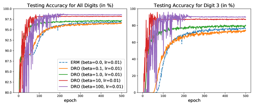
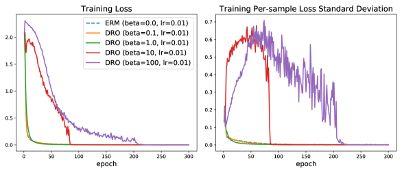
Figure 2: Experiments on MNIST. We compare the learning curves at testing (top panels) and at training (bottom panels) for ERM with SGD (blue) and DRO with our SGD with hardness weighted sampling for different values of (, , , ). The models are trained on an imbalanced MNIST dataset (only of the digits kept for training) and evaluated on the original MNIST testing dataset.
Results:
Our experiment suggests that DRO and ERM lead to different optima. Indeed, DRO for outperforms ERM by more than of accuracy on the underrepresented class, as illustrated in Figure 2. This suggests that DRO is more robust than ERM to domain gaps between the training and the testing dataset. In addition, Figure 2 suggests that DRO with our SGD with hardness weighted sampling can converge faster than ERM with SGD.
Furthermore, the variations of learning curves with shown in Figure 2 are consistent with our theoretical insight. As decreases to , the learning curve of DRO with our Algorithm 1 converges to the learning curve of ERM with SGD.
For large values of (here ), instabilities appear before convergence in the testing learning curves, as illustrated in the top panels of Figure 2. However, the bottom left panel of Figure 2 shows that the training loss curves for were stable there. We also observe that during iterations where instabilities appear on the testing set, the standard deviation of the per-example loss on the training set is relatively high (i.e. the hardness weighted probability is further away from the uniform distribution). This suggests that the apparent instabilities on the testing set are related to differences between the distributionally robust loss and the mean loss.
4.2 Medical Image Segmentation
In this section, we illustrate the application of Algorithm 1 to improve the robustness of deep learning methods for medical image segmentation. We first discuss the specificities of applying the proposed hardness weighted sampling to medical image segmentation in relation to the use of patch-based sampling. We evaluated the proposed method on two applications: fetal brain 3D MRI segmentation using the FeTA dataset and a private dataset, and brain tumor multi-sequence MRI segmentation using the BraTS 2019 dataset (Bakas et al., 2017a, b).
4.2.1 Hardness Weighted Sampler with Large Images
In medical image segmentation, the image used as input of the deep neural network are typically large 3D volumes. For this reason, state-of-the-art deep learning pipelines use patch-based sampling rather than full-volume sampling during training with ERM (Isensee et al., 2021) as described in subsection 4.2.2.
This raised the question of what is the training distribution in the ERM (1) and DRO (3) optimization problems. Here, since the patches are large enough to cover most of the brains, we consider that patches are good approximation of the whole volumes and is the distribution of the full volumes. Therefore, in the hardness weighted sampler of Algorithm 1, we have only one weight per full volume.
In the case the full volumes are too large to be well covered by the patches, one can divide each full volume into a finite number of subvolumes prior to training. For example, for chest CT, one can divide the volumes into left and right lungs (Tilborghs et al., 2020).
4.2.2 Material
Fetal Brain Dataset.
Table 1: Training and Testing Fetal Drain 3D MRI Dataset Details. Other Abn: brain structural abnormalities other than spina bifida. There is no overlap of subjects between training and testing.
Train/Test
Origin
Condition
Volumes
Gestational age (in weeks)
Training
Atlas
Control
18
[21, 38]
Training
FeTA
Control
5
[22, 28]
Training
UHL
Control
116
[20, 35]
Training
UHL
Spina Bifida
28
[22, 34]
Training
UHL
Other Abn
10
[23, 35]
Testing
FeTA
Control
31
[20, 34]
Testing
FeTA
Spina Bifida
38
[21, 31]
Testing
FeTA
Other Abn
16
[20, 34]
Testing
UHL
Control
76
[22, 37]
Testing
UHL and MUV
Spina Bifida
74
[19, 35]
Testing
UHL
Other Abn
25
[21, 40]
A total of (resp. ) fetal brain 3D MRIs were used for training (resp. testing). Origin, condition, and gestational ages for the training and testing datasets are summarized in Table 1.
We used the 18 control fetal brain 3D MRIs of the spatio-temporal fetal brain atlas111http://crl.med.harvard.edu/research/fetal_brain_atlas/ (Gholipour et al., 2017) for gestational ages ranging from weeks to weeks. We also used volumes from the publicly available FeTA MICCAI challenge dataset222DOI: 10.7303/syn25649159 (Payette et al., 2021, 2022) and the 3D MRIs from the testing set of the first release of the FeTA dataset for which manual segmentations are not publicly available. For those 3D MRIs, manual segmentations and corrections of the segmentations were performed by authors MA and LF to reduce the variability against the published segmentation guidelines that was released with the FeTA dataset (Payette et al., 2021). Part of those corrections were performed as part of our previous work (Fidon et al., 2021a, c) and are publicly available333DOI: 10.5281/zenodo.5148611. Brain masks for the FeTA data were obtained via affine registration using two fetal brain atlases444DOI: 10.7303/syn25887675 (Fidon et al., 2021d; Gholipour et al., 2017).
In addition, we used 3D MRIs from a private dataset. All images in the private dataset were part of routine clinical care and were acquired at University Hospital Leuven (UHL) and Medical University of Vienna (MUW) due to congenital malformations seen on ultrasound. In total, cases with spina bifida aperta, cases with other central nervous system pathologies, and cases with other malformations, though with normal brain, and referred as controls, were included. The gestational age at MRI ranged from weeks to weeks. Some of those 3D MRIs and their manual segmentations were used in previous studies (Emam et al., 2021; Fidon et al., 2021d, a; Mufti et al., 2021). We have started to make fetal brain T2w 3D MRIs publicly available555https://www.cir.meduniwien.ac.at/research/fetal/. For each study, at least three orthogonal T2-weighted HASTE series of the fetal brain were collected on a T scanner using an echo time of ms, a repetition time of ms, with no slice overlap nor gap, pixel size mm to mm, and slice thickness mm to mm. A radiologist attended all the acquisitions for quality control.
The reconstructed fetal brain 3D MRIs were obtained using NiftyMIC (Ebner et al., 2020) a state-of-the-art super resolution and reconstruction algorithm. The volumes were all reconstructed to a resolution of mm isotropic and registered to a fetal brain atlas (Gholipour et al., 2017). The 2D MRIs were also corrected for image intensity bias field as implemented in NiftyMIC. Our pre-processing improves the resolution, and removes motion between neighboring slices and motion artefacts present in the original 2D slices (Ebner et al., 2020). It also facilitates the manual delineation of the fetal brain structures compared to the original 2D slices. We used volumetric brain masks to mask the tissues outside the fetal brain. Those brain masks were obtained using the automatic segmentation methods described in (Ebner et al., 2020; Ranzini et al., 2021).
The labelling protocol used for white matter, intra-axial CSF, and cerebellum is the same as in (Payette et al., 2021). We use the term intra-axial CSF rather than ventricular system because in addition to the lateral ventricles, third ventricle, and forth ventricle, it also contains the cavum septum pellucidum and the cavum vergae that are not part of the ventricular system (Tubbs et al., 2011). The three tissue types were segmented for our private dataset by DE, EVE, FG, LF, MA, NM, and TD under the supervision of MA a paediatric radiologist specialized in fetal brain anatomy, who quality controlled and corrected all manual segmentations.
Brain Tumor Dataset.
We have used the BraTS 2019 dataset because it is the last edition of the BraTS challenge for which information about the image acquisition center is available at the time of writing. The dataset contains the same four MRI sequences (T1, ceT1, T2, and FLAIR) for 448 cases, corresponding to patients with either a high-grade Gliomas or a low-grade Gliomas. All the cases were manually segmented for peritumoral edema, enhancing tumor, and non-enhancing tumor core using the same labeling protocol (Menze et al., 2014; Bakas et al., 2018, 2017c). We split the 323 cases of the BraTS 2019 training dataset into 268 for training and 67 for validation. In addition, the BraTS 2019 validation dataset that contains 125 cases was used for testing.
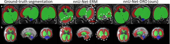
Figure 3: Qualitative Results for Fetal Brain 3D MRI Segmentation using DRO. We have highlighted in white areas with severe violation of the anatomy by nnU-Net-ERM. Most of them are avoided by our nnU-Net-DRO. nnU-Net-ERM and nnU-Net-DRO differ only by the use of the hardness weighted sampler for the latter. a) Fetus with aqueductal stenosis (34 weeks). b) Fetus with spina bifida aperta (27 weeks). c) Fetus with Blake’s pouch cyst (29 weeks). d) Fetus with tuberous sclerosis complex (34 weeks). e) Fetus with spina bifida aperta (22 weeks). f) Fetus with spina bifida aperta (31 weeks). g) Fetus with spina bifida aperta (28 weeks). For cases a) and b), nnU-Net-ERM (Isensee et al., 2021) misses completely the cerebellum and achieves poor segmentation for the white matter and the ventricles. For case c), a large part of the Blake’s pouch cyst is wrongly included in the ventricular system segmentation by nnU-Net-ERM. This is not the case for the proposed nnU-Net-DRO. For case d), nnU-Net-ERM fails to segment the cerebellum correctly and a large part of the cerebellum is segmented as part of the white matter. In contrast, our nnU-Net-DRO correctly segment cerebellum and white matter for this case. For cases e) f) and g), nnU-Net-ERM wrongly included parts of the brainstem in the cerebellum segmentation. nnU-Net-DRO does not make this mistake. We emphasise that the segmentation of the cerebellum for spina bifida aperta is essential for studying and evaluating the effect of surgery in-utero.
Deep Learning Pipeline.
The deep learning pipeline used was based on nnU-Net (Isensee et al., 2021), which is a generic deep learning pipeline for medical image segmentation, that has been shown to outperform other deep learning pipelines on 23 public datasets without the need to manually tune the loss function or the deep neural network architecture. Specifically, we used nnU-Net version 2 in 3D-full-resolution mode which is the recommended mode for isotropic 3D MRI data and the code is publicly available at https://github.com/MIC-DKFZ/nnUNet.
Like most deep learning pipelines in the literature, nnU-Net is based on ERM. For clarity, in the following we will sometimes refer to the unmodified nnU-Net as nnU-Net-ERM.
The meta-parameters used for the deep learning pipeline used were determined automatically using the heuristics developed in nnU-Net (Isensee et al., 2021). The 3D CNN selected for the brain tumor data is based on 3D U-Net (Çiçek et al., 2016) with 5 (resp. 6) levels for fetal brain segmentation (resp. brain tumor segmentation) and 32 features after the first convolution that are multiplied by 2 at each level with a maximum set at 320. The 3D CNN uses leaky activation, instance normalization (Ulyanov et al., 2016), max-pooling downsampling operations and linear upsampling with learnable parameters. In addition, the network is trained using the addition of the mean Dice loss and the cross entropy, and deep supervision (Lee et al., 2015). The default optimization step is SGD with a momentum of and Nesterov update, a batch size of 4 (resp. 2) for fetal brain segmentation (resp. brain tumor segmentation), and a decreasing learning rate defined for each epoch as
where is the maximum number of epochs fixed as . Note that in nnU-Net, one epoch is defined as equal to 250 batches, irrespective of the size of the training dataset. A patch size of (resp. ) was selected for fetal brain segmentation (resp. brain tumor segmentation), which is not sufficient to fit the whole brain of all the cases. As a result, a patch-based approach is used as often in medical image segmentation applications. A large number of data augmentation methods are used: random cropping of a patch, random zoom, gamma intensity augmentation, multiplicative brightness, random rotations, random mirroring along all axes, contrast augmentation, additive Gaussian noise, Gaussian blurring and simulation of low resolution. nnU-Net automatically splits the training data into 5 folds training/ validation. For the experiments on brain tumor segmentation, only the networks corresponding to the first fold were trained. For the experiments on fetal brain segmentation, 5 models were trained, one for each fold, and the predicted class probability maps of the 5 models are averaged at inference to improve robustness (Isensee et al., 2021). GPUs NVIDIA Tesla V100-SXM2 with 16GB of memory were used for the experiments. Training each network took from 4 to 6 days.
Our only modifications of the nnU-Net pipeline is the addition of our hardness weighted sampling when "DRO" is indicated and for some experiments we modified the optimization update rule as indicated in Table 2. Our implementation of the nnU-Net-DRO training procedure is publicly available at https://github.com/LucasFidon/HardnessWeightedSampler. If "ERM" is indicated and nothing is indicated about the optimization update rule, it means that nnU-Net (Isensee et al., 2021) is used without any modification.
Table 2: Evaluation of Distribution Robustness with Respect to the Pathology (260 3D MRIs).nnU-Net-ERM is the unmodified nnU-Net pipeline (Isensee et al., 2021) in which Empirical Risk Minimization (ERM) is used. nnU-Net-DRO is the nnU-Net pipeline modified to use the proposed hardness weighted sampler and in which Distributionally Robust Optimization (DRO) is therefore used. WM: White matter, In-CSF: Intra-axial CSF, Cer: Cerebellum. IQR: interquartile range, : percentile of the Dice score distribution in percentage. Best values are in bold and improvements of at least points of percentage are highlighted.
Dice Score ()
CNS
Method
ROI
Mean
Median
IQR
Controls
nnU-Net-ERM
WM
95.2
2.8
93.3
91.5
90.6
(107 volumes)
(baseline)
In-CSF
90.3
92.4
6.4
87.8
80.7
79.0
Cer
95.7
97.0
3.4
94.2
91.3
90.4
nnU-Net-DRO
WM
94.4
95.3
3.0
93.2
91.1
90.1
(ours)
In-CSF
90.4
92.7
6.2
87.9
81.7
79.1
Cer
95.7
97.1
3.3
94.2
91.4
90.1
Spina Bifida
nnU-Net-ERM
WM
89.6
92.1
4.1
89.5
80.6
73.8
(112 volumes)
(baseline)
In-CSF
91.4
93.9
6.4
89.6
86.9
83.7
Cer
76.8
87.8
11.1
80.4
15.8
0.0
nnU-Net-DRO
WM
90.1
92.2
4.0
89.9
81.6
74.8
(ours)
In-CSF
94.1
6.4
90.0
86.7
83.6
Cer
77.8
87.9
9.7
82.0
43.3
0.0
Other Abn.
nnU-Net-ERM
WM
90.3
92.6
4.6
90.1
88.0
71.6
(41 volumes)
(baseline)
In-CSF
87.4
87.9
10.4
82.7
77.7
75.9
Cer
90.4
92.8
5.4
90.7
87.5
81.4
nnU-Net-DRO
WM
90.4
92.6
4.7
90.2
88.2
73.5
(ours)
In-CSF
87.9
88.1
9.5
83.3
80.4
77.7
Cer
91.3
93.0
5.5
90.7
87.5
82.7
Hyper-parameters of the Hardness Weighted Sampler.
For brain tumor segmentation, we tried the values of with or without importance sampling. Using with importance sampling lead to the best mean dice score on the validation split of the training dataset. For fetal brain segmentation, we tried only with importance sampling. When importance sampling is used, the clipping values and are always used. No other values of and have been tested.
Metrics.
We evaluate the quality of the automatic segmentations using the Dice score (Dice, 1945; Fidon et al., 2017). We are particularly interested in measuring the statistical risk of the results as a way to evaluate the robustness of the different methods.
In the BraTS challenge, this is usually measured using the interquartile range (IQR) which is the difference between the percentiles at and of the the metric values (Bakas et al., 2018). We therefore reported the mean, the median and the IQR of the Dice score in Table 3. For fetal brain segmentation, in addition to the mean, median, and IQR, we also report the percentiles of the Dice score at , , and . In Table 2, we report those quantities for the Dice scores of the three tissue types white matter, intra-axial CSF, and cerebellum.
For each method, nnU-Net is trained 5 times using different train/validation splits and different random initializations. The 5 same splits, computed randomly, are used for the two methods. The results for fetal brain 3D MRI segmentation in Table 2 are for the ensemble of the 5 3D U-Nets. Ensembling is known to increase the robustness of deep learning methods for segmentation (Isensee et al., 2021). It also makes the evaluation less sensitive to the random initialization and to the stochastic optimization.
Table 3: Dice Score Evaluation on the BraTS 2019 Online Validation Set (125 cases). Metrics were computed using the BraTS online evaluation platform (https://ipp.cbica.upenn.edu/). ERM: Empirical Risk Minimization, DRO: Distributionally Robust Optimization, SGD: plain SGD (no momentum used), Nesterov: SGD with Nesterov momentum, IQR: Interquartile range. The best values overall are in bold and improvements of at least points of percentage when comparing ERM and DRO for the same optimizer are highlighted.
Optim.
Optim.
Enhancing Tumor
Whole Tumor
Tumor Core
problem
update
Mean
Median
IQR
Mean
Median
IQR
Mean
Median
IQR
ERM
SGD
71.3
86.0
20.9
90.4
92.3
6.1
80.5
88.8
17.5
DRO
SGD
72.3
87.2
19.1
90.5
92.6
6.0
82.1
89.7
15.2
ERM
Nesterov
73.0
87.1
15.6
90.7
92.6
5.4
83.9
90.5
14.3
DRO
Nesterov
74.5
87.3
13.8
90.6
92.6
5.9
84.1
90.0
12.5
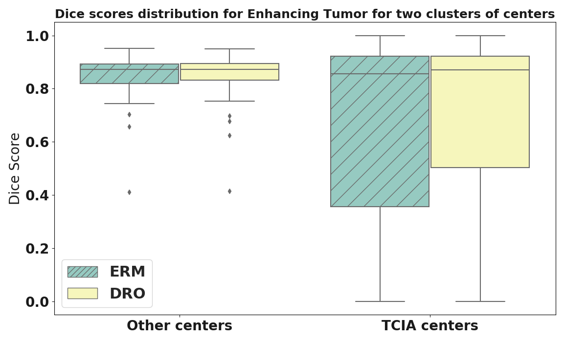
Figure 4: Dice scores distribution on the BraTS 2019 validation dataset for cases from a center of TCIA (76 cases) and cases from other centers (49 cases). This shows that the lower interquartile range of DRO for the enhancing tumor comes specifically from a lower number of poor segmentations on cases coming from The Cancer Imaging Archive (TCIA). This suggests that DRO can deal with some of the confounding biases present in the training dataset, and lead to a model that is more fair.
Results.
The quantitative comparison of nnU-Net-ERM and nnU-Net-DRO on fetal brain 3D MRI segmentation for the three different central nervous system conditions control, spina bifida, and other abnormalities can be found in Table 2.
For spina bifida and other brain abnormalities, the proposed nnU-Net-DRO achieves same or higher mean Dice scores than nnU-Net-ERM (Isensee et al., 2021) with percentage points (pp) for white matter and pp for the cerebellum of spina bifida cases and pp for the cerebellum for other abnormalities. In addition, nnU-Net-DRO achieves comparable (at most pp of difference) or lower IQR than nnU-Net-ERM with pp for the cerebellum of spina bifida cases and pp for the intra-axial CSF of cases with other abnormalities. For controls, the mean, median, and IQR of the Dice scores of nnU-Net-DRO and nnU-Net-ERM differ by less than pp for the three tissue types. This suggests that nnU-Net-DRO is more robust to anatomical variabilities associated with abnormal brains, while retaining the same segmentation performance on neurotypical cases.
In terms of median Dice score, nnU-Net-DRO and nnU-Net-ERM differ by less than pp for all tissue types and conditions. Therefore the differences in terms of mean Dice scores mentioned above are not due to improved segmentation in the middle of the Dice score performance distribution.
The comparison of the percentiles at , , and of the Dice score allows us to compare methods at the tail of the Dice scores distribution where segmentation methods reach their worst-case performance. For spina bifida, nnU-Net-DRO achieves higher values of percentiles than nnU-Net-ERM for the white matter (pp for and pp for ), and for the cerebellum (pp for and pp for ). And for other brain abnormalities, nnU-Net-DRO achieves higher values of percentiles than nnU-Net-ERM for the white matter (pp for ), for the intra-axial CSF (pp for , pp for and pp for ), and for the cerebellum (pp for ). All the other percentile values differ by less than pp of Dice score between the two methods. This suggests that nnU-Net-DRO achieves better worst case performance than nnU-Net-ERM for abnormal cases. However, both methods have a percentile at of the Dice score equal to for the cerebellum of spina bifida cases. This indicates that both methods completely miss the cerebellum for spina bifida cases in of the cases.
As can be seen in the qualitative results of Figure 3, there are cases for which nnU-Net-ERM predicts an empty cerebellum segmentation while nnU-Net-DRO achieves satisfactory cerebellum segmentation. There were no cases for which the converse was true. However, there were also spina bifida cases for which both methods failed to predict the cerebellum. Robust segmentation of the cerebellum for spina bifida is particularly relevant for the evaluation of fetal brain surgery for spina bifida aperta (Aertsen et al., 2019; Danzer et al., 2020; Sacco et al., 2019). All the spina bifida 3D MRIs with missing cerebellum in the automatic segmentations were 3D MRIs from the FeTA dataset Payette et al. (2021) and represented brains of fetuses with spina bifida before they were operated on. The cerebellum is more difficult to detect using MRI before surgery as compared to early or late after surgery (Aertsen et al., 2019; Danzer et al., 2007). No 3D MRI with the combination of those two factors were present in the training dataset (Table. 1). This might explain why DRO did not help improving the segmentation quality for those cases. DRO aims at improving the performance on subgroups that were underrepresented in the training dataset, not subgroups that were not represented at all.
In Table 2, it is worth noting that overall the Dice score values decrease for the white matter and the cerebellum between controls and spina bifida and abnormal cases. It was expected due to the higher anatomical variability in pathological cases. However, the Dice score values for the ventricular system tend to be higher for spina bifida cases than for controls. This can be attributed to the large proportion of spina bifida cases with enlarged ventricles because the Dice score values tend to be higher for larger regions of interest.
For our experiments on brain tumor segmentation, Table 3 summarizes the performance of training nnU-Net using ERM or using DRO. Here, we experiment with two SGD-based optimizers. For both ERM and DRO, the optimization update rule used was either plain SGD without momentum (SGD), or SGD with a Nesterov momentum equal to (Nesterov). Especially, for the latter, this implies that step 12 of Algorithm 1 is modified to use SGD with Nesterov momentum. It was also the case for our experiments on fetal brain 3D MRI segmentation. For DRO, the results presented here are for and using importance sampling (step 6 of Algorithm 1).
As illustrated in Table 3, for both ERM and DRO, the use of SGD with Nesterov momentum outperforms plain-SGD for all metrics and all regions of interest. This result was expected for ERM, for which it is common practice in the deep learning literature to use SGD with a momentum. Our results here suggest that the benefit of using a momentum with SGD is retained for DRO.
For both optimizers, DRO outperforms ERM in terms of IQR for the enhancing tumor and the tumor core by approximately pp of Dice score, and in terms of mean Dice score for the enhancing tumor by pp for the plain-SGD and pp for SGD with Nesterov momentum. For plain-SGD, DRO also outpermforms ERM in terms of mean Dice score for the tumor core by pp. The IQR is the global statistic used in the BraTS challenge to measure the level of robustness of a method (Bakas et al., 2018). In addition, Figure 4 shows that the lower IQR of DRO for the enhancing tumor comes specifically from a lower number of poor segmentations on cases coming from The Cancer Imaging Archive (TCIA). This suggests that DRO can deal with some of the confounding biases present in the training dataset, and lead to a model that is more fair with respect to the acquisition center of the MRI.
Since the same improvements are observed independently of the optimization update rule used. This suggests that in practice Algorithm 1 still converges when a momentum is used, even if Theorem 6 was only demonstrated to hold for plain-SGD.
The value and the use of importance sampling was selected based on the mean Dice score on the validation split of the training dataset. Results for with Nesterov momentum and with or without importance sampling can be found in Appendix B Table 5. The tendency described previously still holds true for the enhancing tumor for equal to or with and without importance sampling. The mean Dice score is improved by pp to pp and the IQR is reduced by pp to pp for the four DRO models as compared to the ERM model. For the tumor core with mean and IQR are improved over ERM with and without importance sampling. However, for with importance sampling there was a loss of performance as compared to ERM for the whole tumor. This problem was not observed with without importance sampling. For the other models with equal to or similar Dice score performance similar to the one ERM was observed for the whole tumor. This suggests that overall the use of ERM or DRO does not affect the segmentation performance of the whole tumor. One possible explanation of this is that Dice scores for the whole tumor are already high for almost all cases when ERM is used with a low IQR. In addition, DRO and the hardness weighted sampler are sensitive to the loss function, here the mean-class Dice loss plus cross entropy loss. In the case of brain tumor segmentation, we hypothesise that the loss function is more sensitive to the segmentation performance for the tumor core and the enhancing tumor than for the whole tumor.
When becomes too large () a decrease of the mean and median Dice score for all regions is observed as compared to ERM. In this case, DRO tends towards the maximization of the worst-case example only which appears to be unstable using our Algorithm 1. For all values of the use of importance sampling, as described in steps 6-8 of Algorithm 1, improves the IQR of the Dice scores for the enhancing tumor and the tumor core. We therefore recommend to use Algorithm 1 with importance sampling.
4.3 Computational Time and Memory Overhead of Algorithm 1
Table 4: Estimated Computational Time and Memory Overhead of the hardness weighted sampler in Algorithm 1. The times (in seconds) are estimated using a batch size of and and by taking the average sampling time over sampling operations for each number of samples. It is worth noting that the sampling operations are computed on the CPUs as in most deep learning pipeline. The time and memory overhead of the proposed hardness weighted sampler is negligible for training datasets with up to 1 million samples.
# Samples
Time (in sec)
Memory (in MB)
7.6
76.3
The main additional computational cost in Algorithm 1 is due to the hardness weighted sampling in steps 4 and 5 that is dependent on the number of training examples. In Table 4, we have computed the computational time and memory overhead of the hardness weighted sampler for different sizes of the training dataset. We have computed that additional time required is less than second and the additional memory less than MB for up to using a batch size of and the function random.choice of Numpy version . The times were estimated using Intel(R) Core(TM) i7-8750H CPU @ 2.20GHz. The additional time and memory that occurs due to the proposed hardness weighted sampling is therefore negligible for all the datasets used in practice in medical image segmentation. For our brain tumor segmentation training set of n=268 volumes and a batch size of 2, the additional memory usage of Algorithm 1 is only 2144 bytes of memory (one float array of size n) and the additional computational time is approximately seconds per iteration using the Python library numpy, i.e. approximately of the total duration of an iteration. The size of the training dataset for fetal brain 3D MRI segmentation being lower, the additional memory usage and the additional computational time are even lower than for brain tumor segmentation. We have made available a python script in our GitHub repository that allows to easily compute the additional time and memory occurring because of the hardness weighted sampler for any number of samples and batch size.
5 Discussion and Conclusion
In this paper, we have shown that efficient training of deep neural networks with Distributionally Robust Optimization (DRO) with a -divergence is possible.
The proposed hardness weighted sampler for training a deep neural network with Stochastic Gradient Descent (SGD) for DRO is as straightforward to implement, and as computationally efficient as SGD for Empirical Risk Minimization (ERM). It can be used for deep neural networks with any activation function (including ), and with any per-example loss function. We have shown that the proposed approach can formally be described as a principled Hard Example Mining strategy (Theorem 7) and is related to minimizing the percentile of the per-example loss distribution (13). In addition, we prove the convergence of our method for over-parameterized deep neural networks (Theorem 6). Thereby, extending the convergence theory of deep learning of Allen-Zhu et al. (2019a). This is, to the best of our knowledge, the first convergence result for training a deep neural network based on DRO.
In practice, we have shown that our hardness weighted sampling method can be easily integrated in a state-of-the-art deep learning framework for medical image segmentation. Interestingly, the proposed algorithm remains stable when SGD with momentum is used. The hardness weighted sampling has one hyperparameter . Our experiments suggest that similar values of lead to improve robustness in different applications. We hypothesize that good values of are of the order of the inverse of the standard deviation of the vector of per-volume (stale) losses during the training epochs that precede convergence.
The high anatomical variability of the developing fetal brain across gestational ages and pathologies hampers the robustness of deep neural networks trained by maximizing the average per-volume performance. Specifically, it limits the generalization of deep neural networks to abnormal cases for which few cases are available during training. In this paper, we propose to mitigate this problem by training deep neural networks using Distributionally Robust Optimization (DRO) with the proposed hardness weighted sampling. We have validated the proposed training method on a multi-centric dataset of fetal brain T2w 3D MRIs with various diagnostics. nnU-Net trained with DRO achieved improved segmentation results for pathological cases as compared to the unmodified nnU-Net, while achieving similar segmentation performance for the neurotypical cases. Those results suggest that nnU-Net trained with DRO is more robust to anatomical variabilities than the original nnU-Net that is trained with ERM. In addition, we have performed experiments on the open-source multiclass brain tumor segmentation dataset BraTS (Bakas et al., 2018). Our results on BraTS suggests that DRO can help improving the robustness of deep neural network for segmentation to variations in the acquisition protocol of the images.
However, we have also found in our experiments that all deep learning models, either trained with ERM or DRO, failed in some cases. For example, the models evaluated all missed the cerebellum in at least of the spina bifida aperta cases. As a result, while our results do suggest that DRO with our method can improve the robustness of deep neural networks for segmentation, they also show that DRO alone with our method does not provide a guarantee of robustness. DRO with a -divergence reweights the examples in the training dataset but cannot account for subsets of the true distribution that are not represented at all in the training dataset. We investigate this problem in our following work (Fidon et al., 2022).
We have shown that the additional computational cost of the proposed hardness weighted sampling is small enough to be negligible in practice and requires less than one second for up to examples. The proposed Algorithm 1 is therefore as computationally efficient as state-of-the-art deep learning pipeline for medical image segmentation. However, when data augmentation is used, an infinite number of training examples is virtually available. We mitigate this problem using importance sampling and only one probability per non-augmented example. We found that importance sampling led to improved segmentation results.
We have also illustrated in our experiments that reporting the mean and standard deviation of the Dice score is not enough to evaluate the robustness of deep neural networks for medical image segmentation. A stratification of the evaluation is required to assess for which subgroups of the population and for which image protocols a deep learning model for segmentation can be safely used. In addition, not all improvements of the mean and standard deviation of the Dice score are equally relevant as they can result from improvements of either the best or the worst segmentation cases. Regarding the robustness of automatic segmentation methods across various conditions, one is interested in improvements of segmentation metrics in the tail of the distribution that corresponds to the worst segmentation cases. To this end, one can report the interquartile range (IQR) and measures of risk such as percentiles.
Acknowledgments
This project has received funding from the European Union’s Horizon 2020 research and innovation program under the Marie Skłodowska-Curie grant agreement TRABIT No 765148; Wellcome [203148/Z/16/Z; WT101957], EPSRC [NS/A000049/1; NS/A000027/1]. Tom Vercauteren is supported by a Medtronic / RAEng Research Chair [RCSRF1819\7\34]. Data used in this publication were obtained as part of the RSNA-ASNR-MICCAI Brain Tumor Segmentation (BraTS) Challenge project through Synapse ID (syn25829067).
Ethical Standards
The work follows appropriate ethical standards in conducting research and writing the manuscript, following all applicable laws and regulations regarding treatment of human subjects.
Conflicts of Interest
Sébastien Ourselin is co-founder of Brainminer and non-executive director at Hypervision Surgical. Tom Vercauteren is chief scientific officer at Hypervision Surgical. Michael Ebner is chief executive officer at Hypervision Surgical. Georg Langs is chief scientist and co-founder at Contextflow.
References
Aertsen et al. (2019) M Aertsen, J Verduyckt, F De Keyzer, T Vercauteren, F Van Calenbergh, L De Catte, S Dymarkowski, P Demaerel, and J Deprest. Reliability of MR imaging–based posterior fossa and brain stem measurements in open spinal dysraphism in the era of fetal surgery. American Journal of Neuroradiology, 40(1):191–198, 2019.
Allen-Zhu et al. (2019a) Zeyuan Allen-Zhu, Yuanzhi Li, and Zhao Song. A convergence theory for deep learning via over-parameterization. In ICML, pages 242–252, 2019a.
Allen-Zhu et al. (2019b) Zeyuan Allen-Zhu, Yuanzhi Li, and Zhao Song. On the convergence rate of training recurrent neural networks. In Advances in Neural Information Processing Systems 32, pages 6676–6688. Curran Associates, Inc., 2019b.
Bakas et al. (2017a) Spyridon Bakas, Hamed Akbari, Aristeidis Sotiras, Michel Bilello, Martin Rozycki, Justin S Kirby, John B Freymann, Keyvan Farahani, and Christos Davatzikos. Segmentation labels and radiomic features for the pre-operative scans of the TCGA-GBM collection. The Cancer Imaging Archive, 2017a. doi: 10.7937/K9/TCIA.2017.KLXWJJ1Q.
Bakas et al. (2017b) Spyridon Bakas, Hamed Akbari, Aristeidis Sotiras, Michel Bilello, Martin Rozycki, Justin S Kirby, John B Freymann, Keyvan Farahani, and Christos Davatzikos. Segmentation labels and radiomic features for the pre-operative scans of the TCGA-LGG collection. The Cancer Imaging Archive, 2017b. doi: 10.7937/K9/TCIA.2017.GJQ7R0EF.
Bakas et al. (2017c) Spyridon Bakas, Hamed Akbari, Aristeidis Sotiras, Michel Bilello, Martin Rozycki, Justin S Kirby, John B Freymann, Keyvan Farahani, and Christos Davatzikos. Advancing the cancer genome atlas glioma MRI collections with expert segmentation labels and radiomic features. Scientific data, 4:170117, 2017c.
Bakas et al. (2018) Spyridon Bakas, Mauricio Reyes, Andras Jakab, Stefan Bauer, Markus Rempfler, Alessandro Crimi, Russell Takeshi Shinohara, Christoph Berger, Sung Min Ha, Martin Rozycki, et al. Identifying the best machine learning algorithms for brain tumor segmentation, progression assessment, and overall survival prediction in the BRATS challenge. arXiv preprint arXiv:1811.02629, 2018.
Berger et al. (2018) Lorenz Berger, Hyde Eoin, M Jorge Cardoso, and Sébastien Ourselin. An adaptive sampling scheme to efficiently train fully convolutional networks for semantic segmentation. In Annual Conference on Medical Image Understanding and Analysis, pages 277–286. Springer, 2018.
Bottou et al. (2018) Léon Bottou, Frank E Curtis, and Jorge Nocedal. Optimization methods for large-scale machine learning. Siam Review, 60(2):223–311, 2018.
Byrd and Lipton (2019) Jonathon Byrd and Zachary Lipton. What is the effect of importance weighting in deep learning? In ICML, pages 872–881, 2019.
Cao and Gu (2020) Yuan Cao and Quanquan Gu. Generalization error bounds of gradient descent for learning overparameterized deep relu networks. In AAAI, 2020.
Chang et al. (2017) Haw-Shiuan Chang, Erik Learned-Miller, and Andrew McCallum. Active bias: Training more accurate neural networks by emphasizing high variance samples. In Advances in Neural Information Processing Systems, pages 1002–1012, 2017.
Chernoff et al. (1952) Herman Chernoff et al. A measure of asymptotic efficiency for tests of a hypothesis based on the sum of observations. The Annals of Mathematical Statistics, 23(4):493–507, 1952.
Chouzenoux et al. (2019) Emilie Chouzenoux, Henri Gérard, and Jean-Christophe Pesquet. General risk measures for robust machine learning. Foundations of Data Science, 1:249, 2019.
Çiçek et al. (2016) Özgün Çiçek, Ahmed Abdulkadir, Soeren S Lienkamp, Thomas Brox, and Olaf Ronneberger. 3D U-Net: learning dense volumetric segmentation from sparse annotation. In International conference on medical image computing and computer-assisted intervention, pages 424–432. Springer, 2016.
Csiszár et al. (2004) Imre Csiszár, Paul C Shields, et al. Information theory and statistics: A tutorial. Foundations and Trends® in Communications and Information Theory, 1(4):417–528, 2004.
Danzer et al. (2007) Enrico Danzer, Mark P Johnson, Michael Bebbington, Erin M Simon, R Douglas Wilson, Larrissa T Bilaniuk, Leslie N Sutton, and N Scott Adzick. Fetal head biometry assessed by fetal magnetic resonance imaging following in utero myelomeningocele repair. Fetal diagnosis and therapy, 22(1):1–6, 2007.
Danzer et al. (2020) Enrico Danzer, Luc Joyeux, Alan W Flake, and Jan Deprest. Fetal surgical intervention for myelomeningocele: lessons learned, outcomes, and future implications. Developmental Medicine & Child Neurology, 62(4):417–425, 2020.
Dice (1945) Lee R Dice. Measures of the amount of ecologic association between species. Ecology, 26(3):297–302, 1945.
Duchi et al. (2016) John Duchi, Peter Glynn, and Hongseok Namkoong. Statistics of robust optimization: A generalized empirical likelihood approach. arXiv preprint arXiv:1610.03425, 2016.
Ebner et al. (2020) Michael Ebner, Guotai Wang, Wenqi Li, Michael Aertsen, Premal A Patel, Rosalind Aughwane, Andrew Melbourne, Tom Doel, Steven Dymarkowski, Paolo De Coppi, et al. An automated framework for localization, segmentation and super-resolution reconstruction of fetal brain MRI. NeuroImage, 206:116324, 2020.
Emam et al. (2021) Doaa Emam, Michael Aertsen, Lennart Van der Veeken, Lucas Fidon, Prachi Patkee, Vanessa Kyriakopoulou, Luc De Catte, Francesca Russo, Philippe Demaerel, Tom Vercauteren, et al. Longitudinal evaluation of brain development in fetuses with congenital diaphragmatic hernia on mri: an original research study. 2021.
European Commission (2019) European Commission. Ethics guidelines for trustworthy AI. Report, European Commission, 2019.
Fenchel (1949) Werner Fenchel. On conjugate convex functions. Canadian Journal of Mathematics, 1(1):73–77, 1949.
Fidon et al. (2017) Lucas Fidon, Wenqi Li, Luis C Garcia-Peraza-Herrera, Jinendra Ekanayake, Neil Kitchen, Sébastien Ourselin, and Tom Vercauteren. Generalised Wasserstein dice score for imbalanced multi-class segmentation using holistic convolutional networks. In International MICCAI Brainlesion Workshop, pages 64–76. Springer, 2017.
Fidon et al. (2021a) Lucas Fidon, Michael Aertsen, Doaa Emam, Nada Mufti, Frédéric Guffens, Thomas Deprest, Philippe Demaerel, Anna L David, Andrew Melbourne, Sébastien Ourselin, et al. Label-set loss functions for partial supervision: Application to fetal brain 3D MRI parcellation. arXiv preprint arXiv:2107.03846, 2021a.
Fidon et al. (2021b) Lucas Fidon, Michael Aertsen, Nada Mufti, Thomas Deprest, Doaa Emam, Frédéric Guffens, Ernst Schwartz, Michael Ebner, Daniela Prayer, Gregor Kasprian, et al. Distributionally robust segmentation of abnormal fetal brain 3D MRI. In Uncertainty for Safe Utilization of Machine Learning in Medical Imaging, and Perinatal Imaging, Placental and Preterm Image Analysis, pages 263–273. Springer, 2021b.
Fidon et al. (2021c) Lucas Fidon, Michael Aertsen, Suprosanna Shit, Philippe Demaerel, Sébastien Ourselin, Jan Deprest, and Tom Vercauteren. Partial supervision for the FeTA challenge 2021. arXiv preprint arXiv:2111.02408, 2021c.
Fidon et al. (2021d) Lucas Fidon, Elizabeth Viola, Nada Mufti, Anna David, Andrew Melbourne, Philippe Demaerel, Sebastien Ourselin, Tom Vercauteren, Jan Deprest, and Michael Aertsen. A spatio-temporal atlas of the developing fetal brain with spina bifida aperta. Open Research Europe, 2021d.
Fidon et al. (2022) Lucas Fidon, Michael Aertsen, Florian Kofler, Andrea Bink, Anna L David, Thomas Deprest, Doaa Emam, Frédéric Guffens, András Jakab, Gregor Kasprian, et al. A Dempster-Shafer approach to trustworthy AI with application to fetal brain MRI segmentation. arXiv preprint arXiv:2204.02779, 2022.
Gholipour et al. (2017) Ali Gholipour, Caitlin K Rollins, Clemente Velasco-Annis, Abdelhakim Ouaalam, Alireza Akhondi-Asl, Onur Afacan, Cynthia M Ortinau, Sean Clancy, Catherine Limperopoulos, Edward Yang, et al. A normative spatiotemporal MRI atlas of the fetal brain for automatic segmentation and analysis of early brain growth. Scientific reports, 7(1):1–13, 2017.
Harwood et al. (2017) Ben Harwood, BG Kumar, Gustavo Carneiro, Ian Reid, Tom Drummond, et al. Smart mining for deep metric learning. In Proceedings of the IEEE International Conference on Computer Vision, pages 2821–2829, 2017.
Hiriart-Urruty and Lemaréchal (2013) Jean-Baptiste Hiriart-Urruty and Claude Lemaréchal. Convex analysis and minimization algorithms I: Fundamentals, volume 305. Springer science & business media, 2013.
Hu and et al (2018) Weihua Hu and et al. Does distributionally robust supervised learning give robust classifiers? In ICML, 2018.
Isensee et al. (2021) Fabian Isensee, Paul F Jaeger, Simon AA Kohl, Jens Petersen, and Klaus H Maier-Hein. nnU-Net: a self-configuring method for deep learning-based biomedical image segmentation. Nature Methods, 18(2):203–211, 2021.
Jin et al. (2019) Chi Jin, Praneeth Netrapalli, and Michael I Jordan. Minmax optimization: Stable limit points of gradient descent ascent are locally optimal. arXiv preprint arXiv:1902.00618, 2019.
Kahn and Marshall (1953) Herman Kahn and Andy W Marshall. Methods of reducing sample size in Monte Carlo computations. Journal of the Operations Research Society of America, 1(5):263–278, 1953.
Larrazabal et al. (2020) Agostina J Larrazabal, Nicolás Nieto, Victoria Peterson, Diego H Milone, and Enzo Ferrante. Gender imbalance in medical imaging datasets produces biased classifiers for computer-aided diagnosis. Proceedings of the National Academy of Sciences, 117(23):12592–12594, 2020.
LeCun (1998) Yann LeCun. The MNIST database of handwritten digits. http://yann. lecun. com/exdb/mnist/, 1998.
Lee et al. (2015) Chen-Yu Lee, Saining Xie, Patrick Gallagher, Zhengyou Zhang, and Zhuowen Tu. Deeply-supervised nets. In Artificial intelligence and statistics, pages 562–570, 2015.
Lin et al. (2019) Tianyi Lin, Chi Jin, and Michael I Jordan. On gradient descent ascent for nonconvex-concave minimax problems. arXiv preprint arXiv:1906.00331, 2019.
Loshchilov and Hutter (2016) Ilya Loshchilov and Frank Hutter. Online batch selection for faster training of neural networks. ICLR Workshop, 2016.
Menze et al. (2014) Bjoern H Menze, Andras Jakab, Stefan Bauer, Jayashree Kalpathy-Cramer, Keyvan Farahani, Justin Kirby, Yuliya Burren, Nicole Porz, Johannes Slotboom, Roland Wiest, et al. The multimodal brain tumor image segmentation benchmark (brats). IEEE transactions on medical imaging, 34(10):1993–2024, 2014.
Moreau (1965) Jean-Jacques Moreau. Proximité et dualité dans un espace hilbertien. Bulletin de la Société mathématique de France, 93:273–299, 1965.
Mufti et al. (2021) Nada Mufti, Michael Aertsen, Michael Ebner, Lucas Fidon, Premal Patel, Muhamad Bin Abdul Rahman, Yannick Brackenier, Gregor Ekart, Virginia Fernandez, Tom Vercauteren, et al. Cortical spectral matching and shape and volume analysis of the fetal brain pre-and post-fetal surgery for spina bifida: a retrospective study. Neuroradiology, pages 1–14, 2021.
Namkoong and Duchi (2016) Hongseok Namkoong and John C Duchi. Stochastic gradient methods for distributionally robust optimization with f-divergences. In Advances in Neural Information Processing Systems, pages 2208–2216, 2016.
Oakden-Rayner et al. (2020) Luke Oakden-Rayner, Jared Dunnmon, Gustavo Carneiro, and Christopher Ré. Hidden stratification causes clinically meaningful failures in machine learning for medical imaging. In Proceedings of the ACM conference on health, inference, and learning, pages 151–159, 2020.
Owen and Zhou (2000) Art Owen and Yi Zhou. Safe and effective importance sampling. Journal of the American Statistical Association, 95(449):135–143, 2000.
Payette et al. (2021) Kelly Payette, Priscille de Dumast, Hamza Kebiri, Ivan Ezhov, Johannes C Paetzold, Suprosanna Shit, Asim Iqbal, Romesa Khan, Raimund Kottke, Patrice Grehten, et al. An automatic multi-tissue human fetal brain segmentation benchmark using the fetal tissue annotation dataset. Scientific Data, 8(1):1–14, 2021.
Payette et al. (2022) Kelly Payette, Hongwei Li, Priscille de Dumast, Roxane Licandro, Hui Ji, Md Mahfuzur Rahman Siddiquee, Daguang Xu, Andriy Myronenko, Hao Liu, Yuchen Pei, et al. Fetal brain tissue annotation and segmentation challenge results. arXiv preprint arXiv:2204.09573, 2022.
Puyol-Antón et al. (2021) Esther Puyol-Antón, Bram Ruijsink, Stefan K Piechnik, Stefan Neubauer, Steffen E Petersen, Reza Razavi, and Andrew P King. Fairness in cardiac mr image analysis: An investigation of bias due to data imbalance in deep learning based segmentation. In International Conference on Medical Image Computing and Computer-Assisted Intervention, pages 413–423. Springer, 2021.
Rafique et al. (2018) Hassan Rafique, Mingrui Liu, Qihang Lin, and Tianbao Yang. Non-convex min-max optimization: Provable algorithms and applications in machine learning. arXiv preprint arXiv:1810.02060, 2018.
Rahimian and Mehrotra (2019) Hamed Rahimian and Sanjay Mehrotra. Distributionally robust optimization: A review. arXiv preprint arXiv:1908.05659, 2019.
Ranzini et al. (2021) Marta Ranzini, Lucas Fidon, Sébastien Ourselin, Marc Modat, and Tom Vercauteren. MONAIfbs: MONAI-based fetal brain MRI deep learning segmentation. arXiv preprint arXiv:2103.13314, 2021.
Sacco et al. (2019) Adalina Sacco, Fred Ushakov, Dominic Thompson, Donald Peebles, Pranav Pandya, Paolo De Coppi, Ruwan Wimalasundera, George Attilakos, Anna Louise David, and Jan Deprest. Fetal surgery for open spina bifida. The Obstetrician & Gynaecologist, 21(4):271, 2019.
Sagawa et al. (2020) Shiori Sagawa, Pang Wei Koh, Tatsunori B Hashimoto, and Percy Liang. Distributionally robust neural networks for group shifts: On the importance of regularization for worst-case generalization. ICLR, 2020.
Shrivastava et al. (2016) Abhinav Shrivastava, Abhinav Gupta, and Ross Girshick. Training region-based object detectors with online hard example mining. In Proceedings of the IEEE conference on computer vision and pattern recognition, pages 761–769, 2016.
Sinha et al. (2018) Aman Sinha, Hongseok Namkoong, and John Duchi. Certifying some distributional robustness with principled adversarial training. ICLR, 2018.
Staib and Jegelka (2017) Matthew Staib and Stefanie Jegelka. Distributionally robust deep learning as a generalization of adversarial training. In NIPS workshop on Machine Learning and Computer Security, 2017.
Suh et al. (2019) Yumin Suh, Bohyung Han, Wonsik Kim, and Kyoung Mu Lee. Stochastic class-based hard example mining for deep metric learning. In Proceedings of the IEEE Conference on Computer Vision and Pattern Recognition, pages 7251–7259, 2019.
Tilborghs et al. (2020) Sofie Tilborghs, Ine Dirks, Lucas Fidon, Siri Willems, Tom Eelbode, Jeroen Bertels, Bart Ilsen, Arne Brys, Adriana Dubbeldam, Nico Buls, et al. Comparative study of deep learning methods for the automatic segmentation of lung, lesion and lesion type in CT scans of COVID-19 patients. arXiv preprint arXiv:2007.15546, 2020.
Tubbs et al. (2011) R Shane Tubbs, Sanjay Krishnamurthy, Ketan Verma, Mohammadali M Shoja, Marios Loukas, Martin M Mortazavi, and Aaron A Cohen-Gadol. Cavum velum interpositum, cavum septum pellucidum, and cavum vergae: a review. Child’s Nervous System, 27(11):1927–1930, 2011.
Ulyanov et al. (2016) Dmitry Ulyanov, Andrea Vedaldi, and Victor Lempitsky. Instance normalization: The missing ingredient for fast stylization. arXiv preprint arXiv:1607.08022, 2016.
Wachinger et al. (2019) Christian Wachinger, Benjamin Gutierrez Becker, Anna Rieckmann, and Sebastian Pölsterl. Quantifying confounding bias in neuroimaging datasets with causal inference. In International Conference on Medical Image Computing and Computer-Assisted Intervention, pages 484–492. Springer, 2019.
Wu et al. (2017) Chao-Yuan Wu, R Manmatha, Alexander J Smola, and Philipp Krahenbuhl. Sampling matters in deep embedding learning. In Proceedings of the IEEE International Conference on Computer Vision, pages 2840–2848, 2017.
Zagoruyko and Komodakis (2016) Sergey Zagoruyko and Nikos Komodakis. Wide residual networks. In Proceedings of the British Machine Vision Conference (BMVC), pages 87.1–87.12. BMVA Press, 2016.
Zou and Gu (2019) Difan Zou and Quanquan Gu. An improved analysis of training over-parameterized deep neural networks. In Advances in Neural Information Processing Systems 32, pages 2055–2064. Curran Associates, Inc., 2019.
A Summary of the Notations used in the Proofs
For the ease of reading the proofs we first summarize our notations.
A.1 Probability Theory Notations
•
•
Let , and a function, we denote .
•
Let , and a function, we denote .
•
is the uniform training data distribution, i.e. .
A.2 Machine Learning Notations
•
n is the number of training examples.
•
d is the dimension of the output.
•
is the dimension of the input.
•
m is the number of nodes in each layer.
•
Training data: , where for all , and .
•
is the predictor (deep neural network).
•
is the set of parameters of the predictor.
•
For all , is the output of the network for example as a function of .
Forall , is the Distributionally Robust Loss evaluated at , where is the parameter that adjusts the distributionally robustness. For short, we also used the terms distributionally robust loss or just robust loss for .
•
DRO is short for Distributionally Robust Optimisation.
A.4 Miscellaneous
By abuse of notation, and similarly to (Allen-Zhu et al., 2019a), we use the Bachmann-Landau notations to hide constants that do not depend on our main hyper-parameters. Let and be two scalar functions, we note:
B Evaluation of the Influence of on the Segmentation Performance for BraTS
Table 5: Detailed evaluation on the BraTS 2019 online validation set (125 cases). All the models in this table were trained using the default SGD with Nesterov momentum of nnU-Net (Isensee et al., 2021). Dice scores were computed using the BraTS online plateform for evaluation https://ipp.cbica.upenn.edu/. ERM: Empirical Risk Minimization, DRO: Distributionally Robust Optimization, IS: Importance Sampling is used, IQR: Interquartile range. The best values are in bold.
Optimization
Enhancing Tumor
Whole Tumor
Tumor Core
problem
Mean
Median
IQR
Mean
Median
IQR
Mean
Median
IQR
ERM
73.0
87.1
15.6
90.7
92.6
5.4
83.9
90.5
14.3
DRO
74.6
86.8
14.1
90.8
93.0
5.9
83.4
90.7
14.5
DRO IS
75.3
86.0
13.3
90.0
91.9
7.0
82.8
89.1
14.3
DRO
73.4
86.7
14.3
90.6
92.6
6.2
84.5
90.9
13.7
DRO IS
74.5
87.3
13.8
90.6
92.6
5.9
84.1
90.0
12.5
DRO
74.5
84.2
33.0
89.5
91.8
5.9
71.1
87.2
41.1
DRO IS
72.2
85.7
15.0
90.3
92.2
6.3
81.1
89.4
15.1
C Importance Sampling Approximation in Algorithm 1
In this section, we give additional details about the approximation made in the computation of the importance weights (step 9 of Algorithm 1).
Let be the parameters of the neural network , be the stale per-example loss vector, and let be an index in the current batch .
We start from the definition of the importance weight for example and use the formula for the hardness weighted sampling probabilities of Example 1.
(19)
where we have assumed that the two sums of exponentials are approximately equal.
D Proof of Example 1: Formula of the Sampling Probabilities for the KL Divergence
We give here a simple proof of the formula of the sampling probabilities for the KL divergence as -divergence (i.e. )
Proof:
For any , the distributionally robust loss for the KL divergence at is given by
where we have used that inside the function. To simplify the notations, let us denote , and . Thus is, by definition, solution of the optimization problem
(20)
First, let us remark that the function is strictly convex on the non empty closed convex set as a sum of strictly convex functions. This implies that the optimization (20) has a unique solution and as a result is well defined.
We now reformulate the optimization problem (20) as a convex smooth constrained optimization problem by writing the condition as constraints.
(21)
s.t.
There exists a Lagrange multiplier , such that the solution of (21) is characterized by
Let , , and , using (30) and the convexity of , we obtain:
(31)
This proves that is -strongly convex.
is convex, and since is closed and convex, (Hiriart-Urruty and Lemaréchal, 2013). We obtain (28) using Definition 3.
We now show that is Frechet differentiable on . Let .
is strongly-convex, so in particular is strictly convex. This implies that the following optimization problem has a unique solution that we denote .
(32)
In addition, using the notion of subderivative of convex functions (Hiriart-Urruty and Lemaréchal, 2013, Definition 4.1.5 p.39), we have
where we have used (Hiriart-Urruty and Lemaréchal, 2013, Proposition 6.1.2 p.39) for the third equivalence, and (28) for the last equivalence.
As a result, . This implies that admit a gradient at , and
(33)
Since this holds for any , we deduce that is Fréchet differentiable on .
We are now ready to show that is -gradient Lipchitz continuous by using the following lemma (Hiriart-Urruty and Lemaréchal, 2013, Theorem 6.1.2 p.280).
Lemma 9
A necessary and sufficient condition for a convex function to be -strongly convex on a convex set is that for all
Using this lemma for , , and , we obtain:
For all , for all , ,
In addition, for , .
And using Cauchy Schwarz inequality
We conclude that
Which implies that is -gradient Lipchitz continuous.
F Proof of Lemma 5: Formula of the Distributionally Robust Loss Gradient
We prove Lemma 5 that we restate here for the ease of reading.
Lemma 10 (Stochastic Gradient of the DRO Loss – Restated from Lemma 5)
For all , we have
(34)
(35)
where is the gradient of with respect to its input.
Proof:
For a given , equality (34) is a special case of (33) for .
G Proof of Theorem 7: Distributionally Robust Optimization as Principled Hard Example Mining
In this section, we demonstrate that the proposed hardness weighted sampling can be interpreted as a principled hard example mining method.
Let an -divergence satisfying Definition 2, and . will play the role of a generic loss vector.
is strongly convex, and is closed and convex, so the following optimization problem has one and only one solution
(36)
Making the constraints associated with explicit, this can be rewritten as
(37)
s.t.
s.t.
There exists KKT multipliers and such that the solution satisfies
(38)
Since is continuously differentiable and strongly convex, we have , where is the Fenchel conjugate of (see Hiriart-Urruty and Lemaréchal, 2013, Proposition 6.1.2). As a result, (38) can be rewritten as
(39)
We now show that the KKT multipliers are uniquely defined.
The ’s are uniquely defined by and :
Since and , for all , either or . In the case and using (39) it comes .
According to Definition 2, is strongly convex and continuously differentiable, so and are continuous and strictly increasing functions. As a result, it exists a unique (dependent to and ) such that:
The KKT multiplier is uniquely defined by and a continuous function of :
Let that satisfies (40). We have . So there exists at least one index such that
Since is continuous and striclty increasing, is continuous and strictly increasing on a neighborhood of . In addition is continuous and increasing, so for all , is a continuous and increasing function.
As a result, is a continuous function that is increasing on , and strictly increasing on a neighborhood of . This implies that is uniquely defined by , and that is continuous.
G.1 Link between Hard Weighted Sampling and Hard Example Mining
For any pseudo loss vector , there exists a unique KKT multiplier and a unique that satisfies (40), so we can define the mapping:
We will now demonstrate that each for is an increasing function of and a decreasing function of the for . Without loss of generality we assume .
Let , and . Let us define , such that and . Similarly as in the proof of the uniqueness of above, we can show that there exists such that the function
is continuous and strictly increasing on , and .
is continuous, so for small enough .
Let us now prove by contradiction that . Therefore, let us assume that . Then, as is an increasing function and is strictly increasing on , and we obtain
which is a contradiction. As a result
(42)
Using equations (40) and (42), and the fact that is an increasing function, we obtain for all
(43)
In addition
So necessarily
(44)
This holds for any and any , which concludes the proof.
H Proof of Equivalence between (17) and (18): Link between DRO and Percentile Loss
In the DRO optimization problem of equation (18), the optimal for any has the closed-form formula as shown in Appendix D
Since the first two terms cancel each other and , we obtain
which is equivalent to the optimization problem (17) because the term above and the term in (17) are independent of
I Proof of Theorem 6: convergence of SGD with Hardness Weighted Sampling for Over-parameterized Deep Neural Networks with ReLU
In this section, we provide the proof of Theorem 6. This generalizes the convergence of SGD for empirical risk minimization in (Allen-Zhu et al., 2019a, Theorem 2) to the convergence of SGD and our proposed hardness weighted sampler for distributionally robust optimization.
We start by describing in details the assumptions made for our convergence result in Section I.1.
In Section I.2, we restate Theorem 6 using the assumptions and notations previously introduced in Section A.
In Section I.3, we give the proof of the convergence theorem. We focus on providing theoretical tools that could be used to generalize any convergence result for ERM using SGD to DRO using SGD with hardness weighted sampling as described in Algorithm 1.
I.1 Assumptions
Our analysis is based on the results developed in (Allen-Zhu et al., 2019a) which is a simplified version of (Allen-Zhu et al., 2019b). Improving on those theoretical results would automatically improve our results as well.
In the following we state our assumptions on the neural network , and the per-example loss function .
Assumption I.1 (Deep Neural Network)
In this section, we use the following notations and assumptions similar to (Allen-Zhu et al., 2019a):
•
h is a fully connected neural network with layers, as activation functions, and nodes in each hidden layer
•
For all , we denote the -dimensional output scores of applied to example of dimension .
•
For all , we denote where is the ground truth associated to example .
•
is the set of parameters of the neural network h, where is the set of weights for layer with , , and for any other .
•
(Data separation) It exists such that for all , if .
•
We assume for some sufficiently large polynomial poly, and . We refer the reader to (Allen-Zhu et al., 2019a) for details about the polynomial poly.
•
The parameters are initialized at random such that:
–
for every
–
for every and
–
for every
Assumption I.2 (Regularity of )
There exists and such that for all i, is a -gradient Lipschitz continuous, -Lipschitz continuous, and bounded (potentially non-convex) function. When the optimization is performed on a closed convex set, the existence of implies that there exists a constant that bounds the gradients of for all i.
I.2 Convergence theorem (restated)
In this section, we restate the convergence Theorem 6 for SGD with hardness weighted sampling and stale per-example loss vector.
As an intermediate step, we will first generalize the convergence of SGD in (Allen-Zhu et al., 2019a, Theorem 2) to the minimization of the distributionally robust loss using SGD and an exact hardness weighted sampling (10), i.e. with an exact per-example loss vector.
Theorem 11 (Convergence with exact per-example loss vector)
Let batch size , and . Under assumption I.1 and assumption I.2, suppose there exists constants such that the number of hidden units satisfies , , and the learning rate be . There exists constants such that with probability at least over the randomness of the initialization and the mini-batches, SGD with hardness weighted sampling and exact per-example loss vector guarantees after iterations.
is a lower bound on the sampling probabilities. For the Kullback-Leibler -divergence, and for any -divergence satisfying Definition 2 with a robustness parameter small enough, we have . We refer the reader to (Allen-Zhu et al., 2019a, Theorem 2) for the values of the constants and the definitions of the polynomials.
Compared to (Allen-Zhu et al., 2019a, Theorem 2) only the learning rate differs. The operation in the formula for allows us to guarantee that where is the learning rate of (Allen-Zhu et al., 2019a, Theorem 2).
It is worth noting that for the KL -divergence, . In addition, in the limit , which corresponds to ERM, we have . As a result, we recover exactly Theorem 2 of (Allen-Zhu et al., 2019a) as extended in their Appendix A for any smooth loss function that satisfies assumption I.2 with .
We now restate the convergence of SGD with hardness weighted sampling and a stale per-example loss vector as in Algorithm 1.
Theorem 12 (Convergence with a stale per-example loss vector)
Let batch size , and . Under the conditions of Theorem 11, the same notations, and with the learning rate for a constant . With probability at least over the randomness of the initialization and the mini-batches, SGD with hardness weighted sampling and stale per-example loss vector guarantees after iterations.
is a constant such that is -Lipschitz continuous, and is a constant that bounds the gradient of with respect to its input. and are guaranteed to exist under assumptions I.1.
Compared to Theorem 11 only the learning rate differs. Similarly to Theorem 11, when tends to zero we recover Theorem 2 of (Allen-Zhu et al., 2019a).
It is worth noting that when increases, decreases. This implies that decreases faster than when increases. This was to be expected since the error that is made by using the stale per-example loss vector instead of the exact loss increases when increases.
I.3 Proofs of convergence
In this section, we prove the results of Therem 11 and 12.
For the ease of reading the proof, we remind here the chain rules for the distributionally robust loss that we are going to use intensively in the following proofs.
Chain rule for the derivative of with respect to the network outputs :
(45)
Chain rule for the derivative of with respect to the network parameters :
(46)
where for all , is the transpose of the Jacobian matrix of as a function of .
I.3.1 Proof that R o L is one-sided gradient Lipchitz
This property that is one-sided gradient Lipschitz is a key element for the proof of the semi-smoothness theorem for the distributionally robust loss Theorem 13.
Under Definition 2 for the -divergence, we have shown that is -gradient Lipchitz continuous (Lemma 4). And under assumption I.2, for all , is -Lipschitz continuous and -gradient Lipschitz continuous.
Let .
We want to show that is one-sided gradient Lipschitz, i.e. we want to prove the existence of a constant , independent to and , such that:
We have
(47)
Where for all we have used the chain rule
Let
For all , is -gradient Lipchitz continuous, so using Cauchy-Schwarz inequality
(48)
Let
Using the triangular inequality:
(49)
Combining equations (47), (48) and (49) we finally obtain
(50)
From there, we can obtain the following inequality that will be used for the proof of the semi-smoothness property in Theorem 13
(51)
I.3.2 Semi-smoothness property of the distributionally robust loss
We prove the following lemma which is a generalization of Theorem 4 in (Allen-Zhu et al., 2019a) for the distributionally robust loss.
Theorem 13 (Semi-smoothness of the distributionally robust loss)
Let , and the being initialized randomly as described in assumption I.1. With probability as least over the initialization, we have for all with , and
(52)
where for all layer , is the vector of parameters for layer , and
To compare this semi-smoothness result to the one in (Allen-Zhu et al., 2019a, Theorem 4), let us first remark that
As a result, our result is analogous to (Allen-Zhu et al., 2019a, Theorem 4), up to an additional multiplicative factor in the last term of the right-hand side. It is worth noting that there is also implicitly an additional multiplicative factor in Theorem 3 of (Allen-Zhu et al., 2019a) since (Allen-Zhu et al., 2019a) make the assumption that (see Allen-Zhu et al., 2019a, Appendix A).
For all , let us denote to match the notations used in (Allen-Zhu et al., 2019a) for the derivative of the loss with respect to the output of the network for example i of the training set.
With this notation, we obtain exactly equation (11.3) in (Allen-Zhu et al., 2019a) up to the multiplicative factor for the distributionally robust loss.
From there the proof of Theorem 4 in (Allen-Zhu et al., 2019a) being independent to the formula for , we can conclude the proof of our Theorem 13 as in (Allen-Zhu et al., 2019a, Appendix A).
I.3.3 Gradient bounds for the distributionally robust loss
We prove the following lemma which is a generalization of Theorem 3 in (Allen-Zhu et al., 2019a) for the distributionally robust loss.
Theorem 14 (Gradient Bounds for the Distributionally Robust Loss)
Let , and being initialized randomly as described in assumption I.1. With probability as least over the initialization, we have for all with
(55)
It is worth noting that the loss vector used for computing the robust probabilities does not have to be equal to .
We will use this for the proof of the Robust SGD with stale per-example loss vector.
The adaptation of the proof of Theorem 3 in (Allen-Zhu et al., 2019a) is straightforward.
Let satisfying the conditions of Theorem 14, and .
Let us denote , applying the proof of Theorem 3 in (Allen-Zhu et al., 2019a) to our gives:
In addition
This allows us to conclude the proof of our Theorem 14.
I.3.4 Convergence of SGD with Hardness Weighted Sampling and exact per-example loss vector
Similarly to the proof of the convergence of SGD for the mean loss (Theorem 2 in (Allen-Zhu et al., 2019a)), the convergence of SGD for the distributionally robust loss will mainly rely on the semi-smoothness property (Theorem 13) and the gradient bound (Theorem 14) that we have proved previously for the distributionally robust loss.
Let satisfying the conditions of Theorem 11, and be the exact per-example loss vector at , i.e.
(56)
For the batch size , let a batch of indices drawn from without replacement, i.e.
(57)
Let be the values of the parameters after a stochastic gradient descent step at for the batch , i.e.
(58)
where is the learning rate.
Assuming that and satisfies the conditions of Theorem 13, we obtain
(59)
where we refer to (46) for the form of and to (45) for the form of .
In addition, we make the assumption that for the set of values of considered the hardness weighted sampling probabilities admit an upper-bound
(60)
Which is always satisfied under assumption I.2 for Kullback-Leibler -divergence, and for any -divergence satisfying Definition 2 with a robustness parameter small enough.
Let be the expectation with respect to . Applying to (59), we obtain
(61)
where we have used the following results:
•
For any integer , and all , we have (see the proof in I.3.5)
It is worth noting in (67) the apparition of defined in (60). If we were using a uniform sampling as for ERM (i.e. for DRO in the limit ), we would have . So although our inequality (67) may seem crude, it is consistent with equation (13.2) in (Allen-Zhu et al., 2019a) and the corresponding inequality in the case of ERM.
The rest of the proof of convergence will consist in proving that dominates the two last terms in (59). As a result, we can already state that either the robustness parameter , or the learning rate will have to be small enough to control .
Indeed, combining (59) with the chain rule (46), and the gradient bound Theorem 14 where we use our defined in (56)
(68)
where we have used
(69)
There are only two differences compared to equation (13.2) in (Allen-Zhu et al., 2019a):
•
in the last fraction we have instead of (see remark I.3.4 for more details), and an additional multiplicative term . So in total, this term differs by a multiplicative factor from the analogous term in the proof of (Allen-Zhu et al., 2019a).
•
we have instead of . In fact they are analogous since in equation (13.2) in (Allen-Zhu et al., 2019a), is the squared norm of the mean loss for the loss. We don’t make such a strong assumption on the choice of (see assumption I.2). It is worth noting that the same analogy is used in (Allen-Zhu et al., 2019a, Appendix A) where they extend their result to the mean loss with other objective function than the loss.
Our choice of learning rate in Theorem 12 can be rewritten as
(70)
And we also have
(71)
where is the learning rate chosen in the proof of Theorem 2 in (Allen-Zhu et al., 2019a). We refer the reader to (Allen-Zhu et al., 2019a) for the details of the constant in "" and the exact form of the polynomial .
As a result, for , the term dominates the other term of the right-hand side of inequality (68) as in the proof of Theorem 2 in (Allen-Zhu et al., 2019a).
This implies that the conditions of Theorem 14 are satisfied for all , and that we have for all iteration
(72)
And using a result in Appendix A of (Allen-Zhu et al., 2019a), since under assumption I.2 the distributionally robust loss is non-convex and bounded, we obtain for all
However, we are interested in a bound on , rather than a bound on . Using the gradient bound of Theorem 14 and the chain rules (46) and (45)
(75)
where is the constant hidden in .
So with , we finally obtain
(76)
If
(77)
which concludes the proof.
I.3.5 Proof of technical lemma 1
For any integer , and all , we have
(78)
I.4 Convergence of SGD with Hardness Weighted Sampling and stale per-example loss vector
The proof of the convergence of Algorithm 1 under the conditions of Theorem 12 follows the same structure as the proof of the convergence of Robust SGD with exact per-example loss vector I.3.4. We will reuse the intermediate results of I.3.4 when possible and focus on the differences between the two proofs due to the inexactness of the per-example loss vector.
Let be the iteration number, and let be the parameters of the deep neural network at iteration . We define the stale per-example loss vector at iteration as
(79)
where for all , corresponds to the latest iteration before at which the per-example loss value for example has been updated. Or equivalently, it corresponds to the last iteration before when example was drawn to be part of a mini-batch.
We also define the exact per-example loss vector that is unknown in Algorithm 1, as
where we are guaranteed that under assumptions I.1.
Since Theorem 14 is independent to the choice of , taking the expectation with respect to , similarly to (68), we obtain
(84)
where the differences with respect to (68) comes from the fact that is not the exact per-example loss vector here, i.e. , which leads to
(85)
and
(86)
Let
(87)
Where is a constant such that is -Lipschitz continuous, and is a constant that bound the gradient of with respect to its input. and are guaranteed to exist under assumptions I.1.
Using assumptions I.2 and (Allen-Zhu et al., 2019a, Claim 11.2)
(96)
Where is the constant of Lipschitz continuity of the per-example loss (see assumptions I.2) and is the constant of Lipschitz continuity of the deep neural network with respect to its parameters .
By developing the recurrence formula of (81), we obtain
Let a bound on the gradient of the per-example loss function. Using Theorem 14 and the chain rule
(97)
And using the triangle inequality
(98)
As a result, we obtain
(99)
For all and for any the probability that the sample is not in batch is lesser than .
Therefore, for any and for any ,
(100)
For , we have , and thus with probability at least ,
(101)
As a result, we finally obtain that with probability at least ,
(102)
I.4.2 Proof of technical lemma 3
Let us first denote
(103)
Using Cauchy-Schwarz inequality
(104)
Let
(105)
Using again Cauchy-Schwarz inequality
(106)
As a result, becomes
(107)
Using the triangular inequality, Theorem 14, and Lemma I.4.1, we finally obtain