1 Introduction
Generative modelling of complex datasets (e.g. images) has advanced greatly in recent years with the advent and development of generative adversarial networks (GANs) (Goodfellow et al., 2014). GANs are a class of deep learning methods that in general pit two networks against each other in a ‘game’ wherein the goal of one network (the discriminator) is to distinguish between real samples and the output from the other network (the generator), while the goal of the generator is to produce samples that are difficult for the discriminator to correctly identify as real or not. By training the two networks in an adversarial fashion, the generator can learn to produce realistic random outputs for even complex data distributions.
GANs have primarily been developed in natural image processing due to the availability of large public datasets, and in that domain they have found particular application in image manipulation, whereby conditioning on an input image allows for non-linear image filtering, scene modification, and attribute switching (Perarnau et al., 2016; Lample et al., 2017; Zhu et al., 2017; Isola et al., 2017).
GANs have also been widely applied in medical imaging, across a range of tasks such as image-to-image translation (including segmentation) (Emami et al., 2018; Dong et al., 2019), advanced data augmentation, (Liu et al., 2018; Frid-Adar et al., 2018; Bu et al., 2021; Barile et al., 2021), image reconstruction and restoration (Reader et al., 2020; Ravishankar et al., 2020; Montalt-Tordera et al., 2021), and anomaly detection (Schlegl et al., 2019). See Yi et al. (2019) for a recent review of GANs in medical imaging.
These latter two problems, anomaly detection (Schlegl et al., 2019) and image reconstruction/restoration (Reader et al., 2020; Ravishankar et al., 2020; Montalt-Tordera et al., 2021), serve as the motivation for this work. For anomaly detection, an accurate model of the entire distribution of healthy images is required to reliably identify new query images as within- or out-of-distribution relative to healthy samples, i.e. to identify them as anomalous or not. For image reconstruction, while GANs are most commonly used in an image-to-image fashion (e.g. for denoising image estimates while preserving realism), they also present the opportunity to learn the entire distribution of valid images, information which can be used as data-driven regularisation (Reader et al., 2020).
Given the potential uses for GAN models that approximate the entire distribution of tissue appearance, adapting them for different applications (e.g. tissue/modality combinations) is of great interest. See Quiros et al. (2021) for an example of the development of a high-quality GAN model in histology imaging.
To summarise, to our knowledge this work is the first to train and evaluate GAN methods to model the appearance of healthy lung tissue in CT images in a fully 3D manner. Due to the extensive research required to produce and evaluate well-performing 3D GAN models that match the training data distribution both in appearance and in semantic features, we leave the evaluation of downstream tasks for future work. In the spirit of open-source biomedical research supporting code for this project is available online111https://github.com/S-Ellis/healthy-lungCT-GANs.
The specific contributions of this work are:
- 1.
we adapt GAN models from the literature to allow 3D output, and investigate their performance on the CT lung patch generation task with the commonly used Fréchet inception distance (FID) metric and an observer study;
- 2.
we propose to use a minibatch discrimination technique (MDmin) and a method of increasing the effective batch size to improve performance over baseline methods;
- 3.
we perform 3D, domain-specific analysis of the generated patches, and relate the 3D structure of output images to the latent space of GAN models; and
- 4.
these results provide baseline performance metric values for the lung CT patch generation task, serving as a reference for future work in this area.
The structure of the rest of this paper is as follows: In Section 2, the principles of GANs are described, along with the details of the specific GAN methods that were employed in this study. Section 3 outlines the experimental set-up, including the data sampling, training process, and the evaluations that were performed. Sections 4 and 5 describe and discuss the results of the experiments and Section 6 summarises the conclusions of this work.
2 Methods
In this work we adapt three GAN generator architectures to the 3D lung CT patch modelling problem: the widely investigated DCGAN (Radford et al., 2016) representing a baseline approach, and styleGAN (Karras et al., 2019) and bigGAN (Brock et al., 2019) approaches which are more representative of the state-of-the-art in generator architectures. It is important to emphasise that these methods could not be used ‘out-of-the-box’ and modification was required to allow 3D patch output. Therefore, we denote the methods investigated in this study as DCGAN3D, styleGAN3D, and bigGAN3D respectively.
In general, a GAN model consists of a generator and a discriminator network . The generator takes as input samples from the prior distribution (usually a normal distribution), and outputs fake images so that with . The discriminator takes as input a minibatch of images from either (or both) the real and fake distributions, with real images denoted by , and returns some per-sample value which provides feedback on the ‘realism’ of . The distribution of real images is denoted and the aim of GAN training is for throughout the training process.
2.1 DCGAN3D generator
The deep convolutional GAN (DCGAN, Radford et al. (2016)) architecture was developed to be able to incorporate convolutions into a GAN model, since the original GAN of Goodfellow et al. (2014) used only fully-connected layers, which limited the size of the output images. The DCGAN3D generator used in this work is described in Appendix A, adapted from the publicly available 2D PyTorch implementation222https://github.com/pytorch/examples/blob/master/dcgan/main.py, accessed Feb 2020. The total number of parameters was million. In summary, the latent code is expanded to a volume via convolution, and then this volume is progressively upsampled with transposed convolution layers until reaching the output size of . Each transposed convolution operation is followed by a 3D batchnorm (Ioffe and Szegedy, 2015) and a ReLU activation, except the last layer which has a tanh activation to bound the generated image in .
2.2 styleGAN3D generator
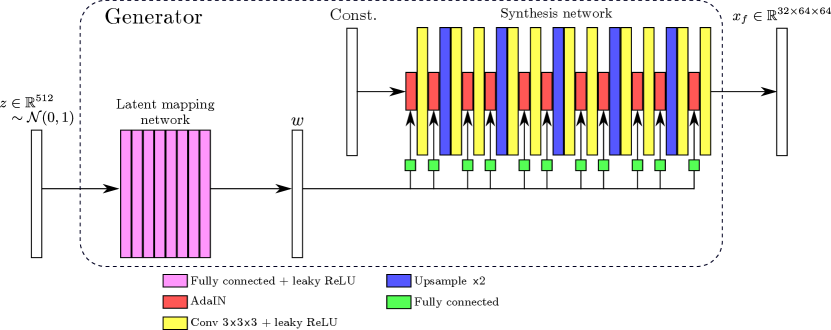
StyleGAN improves on other GAN techniques by using style-based image generation (Karras et al., 2019). The latent code is processed by a set of fully-connected layers and fed into a convolutional generator at multiple resolution scales to control the statistics of the activation maps using adaptive instance normalisation (Huang and Belongie, 2017). This is a more powerful method of altering overall image appearance than learning across multiple convolutional-only layers.
The styleGAN generator also incorporates a mapping network which maps to a another, warped space, which has distribution . The aim is to allow the network to learn a more natural latent space, such that the vectors are better structured according to semantic image features (Karras et al., 2019).
Figure 1 shows schematically the architecture of the 3D styleGAN (styleGAN3D) patch generator implemented in this work, and Appendix B describes the details of the latent mapping and synthesis networks. The total number of trainable parameters was million. Note that in this work the noise injection channels of the original styleGAN architecture were omitted since we would wish to retain control of all relevant details of the generated images for the potential downstream tasks of anomaly detection and image reconstruction.
2.3 bigGAN3D generator
bigGAN is a competing high-quality GAN model first described by Brock et al. (2019). By combining various architectural components that had previously been shown to aid GAN training, and systematically optimising the resulting architectures, bigGAN was demonstrated to allow stable training for high-resolution natural images. In particular, bigGAN inherits spectral normalisation Miyato et al. (2018) and self-attention layers Zhang et al. (2019) from previous GAN models. We adapted the publicly available bigGAN implementation333https://github.com/ajbrock/BigGAN-PyTorch, accessed Mar 2022 to 3D, with the full architecture listed in Appendix C. Note that due to memory constraints the bigGAN3D architecture had only million trainable parameters.
2.4 Discriminator
We used a simple convolutional feed-forward network as the discriminator backbone for all methods, as is common in both older and more recent GAN models (Radford et al., 2016; Karras et al., 2018, 2019). We also used minibatch discrimination (MD) to increase variability of GAN output. MD refers to a family of techniques which can be employed to avoid mode collapse (where many are similar) by allowing the discriminator to make comparisons between samples in a minibatch (Salimans et al., 2016). MD is particularly useful when the discriminator architecture is shallow, since shallow networks are intrinsically less able to detect mode collapse.
In this work we use a minimum-based MD method, denoted MDmin. Full details are given in Appendix D, but in summary the minimum perceptual difference between samples in a minibatch is provided to the discriminator to facilitate inclusion of whole-batch information. When mode-collapse has occurred for a generator model, this measure is small, allowing the discriminator to more easily detect that the minibatch is fake, providing a strong signal to the generator to diversify its samples.
The details of the discriminator architecture, including the location of the MDmin layer are given in Table 1. The number of trainable parameters was million. Note that the MDmin layer is placed just before the final convolutional layer to allow the discriminator to quickly detect the MD signal in cases of mode collapse.
We also note that the effectiveness of minibatch discrimination is limited by the maximum batch size that is computationally feasible. For this reason we use a heuristic trick to increase the effective batch size by pre-selecting the most similar (according to the MDmin) samples from a larger batch of samples, thereby allowing the discriminator to reliably see the most mode-collapsed samples for a particular model. We denote this training heuristic largeEBS (large effective batch size), and a full description is provided in Appendix D.
| Discriminator |
|---|
| Input: |
| Conv3d , stride 2, pad , no bias, 164 |
| Leaky ReLU 0.2 |
| Conv3d , stride 2, pad 1, no bias, 64128 |
| Leaky ReLU 0.2 |
| Conv3d , stride 2, pad 1, no bias, 128256 |
| Leaky ReLU 0.2 |
| Conv3d , stride 2, pad 1, no bias, 256512 |
| Leaky ReLU 0.2 |
| (Optional: MDmin) |
| Conv3d , stride 1, pad 0, no bias, 512/5131 |
| Output: |
2.5 Loss functions
The original seminal work on GANs introduced by Goodfellow et al. (2014) proposed an intuitive approach where the discriminator aims to correctly classify real and fake images, while the generator aims to force the discriminator to misclassify fake images as real. Concretely, the losses for the two networks are:
| (1) |
and
| (2) |
where denotes the sigmoid function. Note that expectation values are defined over the entirety of the distributions, but in practice these losses are calculatated batch-wise as an approximation.
There are many alternative losses that have been proposed for training GANs, including Wasserstein distance (Arjovsky et al., 2017; Gulrajani et al., 2017), least-squares (Mao et al., 2017), Hinge loss (Lim and Ye, 2017), etc. Evaluating all such loss functions for a given application is a time-consuming exercise that we leave for future work. In this work we focus on one of the relativistic losses of Jolicoeur-Martineau (2019), which has been incorporated successfully into large-scale GAN models of medical images (Quiros et al., 2021). The equations for the relativistic losses are:
| (3) |
and
| (4) |
where:
| (5) |
Intuitively, these relativistic losses reframe the task of the discriminator and generator so that the discriminator now aims to assign higher output to real images than for fake ones. The generator then aims to ‘fool’ the discriminator to do the opposite. Note that in this case the generator learns directly from both the fake and real images, whereas for the standard GAN losses (Equations 1 and 2), the generator only receives direct feedback from the discriminator on the fake images.
3 Experiments
3.1 Dataset
We used the publicly available LUNA16 lung CT dataset (Setio et al., 2017), comprising 888 lung CT images, annotated by four radiologists. These annotations include malignancy scores and segmentations for nodules diameter. We chose to exclude nodules and pathological images from the present study to approximate the training of a GAN for a downstream anomaly detection task.
First, we exclude nodules by selectively rejecting sampled patches that contain any ground truth nodule voxels. Second, we considered all scans that had any single nodule with a median malignancy score (across radiologists) as diseased, excluding the whole CT volume from further use. Removing these malignant scans left 636 scans which were split into 509 training scans and 127 held out for future testing.
3.2 Comparative Methods
Using various combinations of the above GAN components results in a number of overall comparison methods for training our GAN. Table 2 summarises the combinations we chose to compare in this work.
| Method abbreviation | Generator type | MDmin | Increased effective batch size |
|---|---|---|---|
| DCGAN3D-base | DCGAN | ✗ | ✗ |
| DCGAN3D-MDmin | DCGAN | ✓ | ✗ |
| DCGAN3D-MDmin-largeEBS | DCGAN | ✓ | ✓ |
| styleGAN3D-base | styleGAN | ✗ | ✗ |
| styleGAN3D-MDmin | styleGAN | ✓ | ✗ |
| styleGAN3D-MDmin-largeEBS | styleGAN | ✓ | ✓ |
| bigGAN3D-base | bigGAN | ✗ | ✗ |
| bigGAN3D-MDmin | bigGAN | ✓ | ✗ |
| bigGAN3D-MDmin-largeEBS | bigGAN | ✓ | ✓ |
3.3 Model Training
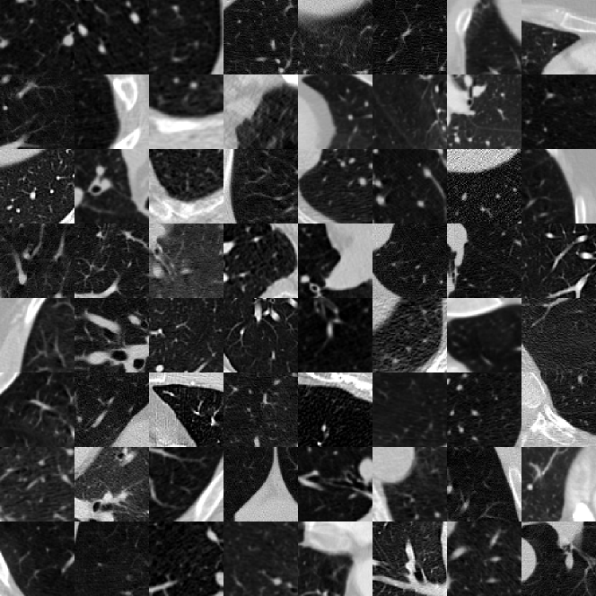
The training of GAN model involves sampling from the real image distribution, as well as generating fake images using the generator. As shown above, the GAN output was of size vox3. Therefore patches sampled from the real CT images were also of this size. Patches were sampled from within the lung using the LUNA16 provided lung masks, excluding all voxels annotated as nodules as described above. Figure 2 show a sample of real patches (centre slice only), highlighting the high variability in lung wall position and vessel structure. Note that resampling to a standard voxel size and other data augmentations (translation, rotation, etc) were not performed.
Unless stated otherwise, for a given CT image, 672 patches were sampled at a time, windowed to HU, and then rescaled to . These patches were then used to create minibatches of size 48, with 14 minibatches per image. For each update of the discriminator, this batch of 48 real images is passed through to obtain , followed by a batch of 48 fake images to get . A similar sampling process is followed for the generator updates. A single pass through all 509 training CT scans (i.e. 7126 iterations) is considered an epoch of training. For each epoch, patches are sampled separately, ensuring that with high probability no single patch is repeated during the training.
For all GAN models, the generator and discriminator learning rates were set the same at , using the Adam optimiser (Kingma and Ba, 2015) with . The discriminator and generator were each updated once per iteration. Training was run for 20 epochs using either an NVIDIA GeForce GTX 1080 Ti or an NVIDIA TITAN Xp GPU.
Finally, for the styleGAN3D approach, so-called style-mixing regularisation was used (Karras et al., 2019) which swaps two latent codes and at a random depth in the convolutional generator. Since the GAN training process still encourages the output to be realistic, the effect is to decouple the effect of the latent code at different scales (see Karras et al. (2019) for further details). Note that in comparison to the standard 2D styleGAN method of Karras et al. (2019), progressive growing of images was not found to be necessary for styleGAN3D due to the small relative size of the output patches compared to the convolutional kernel sizes.
3.4 Automatic Model Evaluation with FID
GAN models were evaluated throughout training with the commonly-used Fréchet inception distance (FID) which was proposed and explained in detail by Heusel et al. (2017). In brief, the FID aims to measure the similarity between the distributions of real training images () and fake, GAN produced images (). To do this, a large number (–) of images from each distribution is sampled. These images are passed through a pre-trained network to obtain the activations at a deep layer, which can be assumed to be Gaussian in distribution. Measuring the Fréchet distance between these two distributions provides a measure of similarity between the original distributions. The FID provides a measure of both average image quality (i.e. ‘realism’) and variability, and so it is sensitive to mode collapse.
As mentioned, FID uses a pre-trained network to provide higher-level representations of the input images. In common practice, this network is an Inception network pre-trained on a natural image task (Heusel et al., 2017), which presents two considerations for use in the current investigation. Firstly, the pre-trained network accepts only 2D input. Therefore, when calculating FID for our 3D GANs, we use only the central slices of generated images. Secondly, since the data domain is different (natural images vs lung CT patches), the transferability of the standard Inception network to lung CT could be questionable. However, we note that calculating the FID between two random sets of real images produces a low FID value of , suggesting that producing a low FID score is a valid target for GAN models of lung CT patches.
We used FID to measure GAN performance throughout training, with five training runs performed for each method listed in Table 2. For each method we selected the lowest-FID model from across the five training runs as the best. These lowest FIDs were then compared between architectures, and the corresponding models were retained for further investigation and characterisation.
3.5 Observer Study
To complement the results of the automated model evaluation, we also performed a human observer study on the best performing 3D GAN models. One human observer (SE) was provided 200 2D image slices per model, split 50:50 into real and fake. The task was to classify real and fake images, and this was repeated three times to assess intra-observer variability. Receiver operating characteristic (ROC) analysis of the results was then performed.
3.6 3D Domain-Specific Analysis
The analyses and model selection described above were performed only in 2D due to the reliance of the standard FID on a 2D Inception network, and the infeasibility of performing large observer studies with 3D patches. To investigate the 3D, domain-specific structure of the generated patches, additional analysis was performed.
Firstly, although the conventional FID measurement uses a trained 2D Inception network, there has been research proposing the use of a 3D network to enable a 3D FID score (Sun et al., 2020). In this case the network from which activations are retrieved is a 3D ResNet pre-trained on different medical imaging segmentation datasets (Chen et al., 2019). Transfer learning experiments showed that the learnt features in such a network were beneficial for a range of tasks, including segmentation of lung tissue in CT images (Chen et al., 2019). We use one model provided by Chen et al. (2019) to calculate a 3D FID (FID3D) for our lung tissue GANs. Specifically, we use a pre-trained ResNet-10 model, and obtain the output activation maps, which have dimensions of when given input. To avoid excessive memory usage we spatially average these maps to obtain a element feature per input patch. Processing real and fake images allows the Fréchet distance to be measured between real and fake datasets as for standard 2D FID.
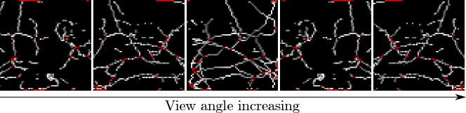
Secondly, we note that if the distributions of real and fake images are close, then we expect that the distributions of any quantity derived from those images should also be close, i.e. comparing the distributions of any characteristic of real and fake images is valid. Beyond this, using a quantity relevant for the task at hand is preferable. To the best of our knowledge, little research has been performed on the expected appearance of healthy lung tissue in CT image patches. Therefore we opted to analyse the appearance of a prominent feature of healthy lung tissue patches: the vasculature. Specifically we chose to model the complexity of the vasculature by finding the number of branch points in an automated fashion. 3D patches were skeletonised using standard python scikit-image library functions in order to provide a sparse representation of the 3D structure. These 3D skeletons were visually assessed using 3D rotating maximum intensity projections (MIPs). The number of branch points was automatically detected, and the distribution of branch points across 10k images was recorded. Figure 3 shows an example skeletonisation of a generated patch, with automatically detected branch-points highlighted.
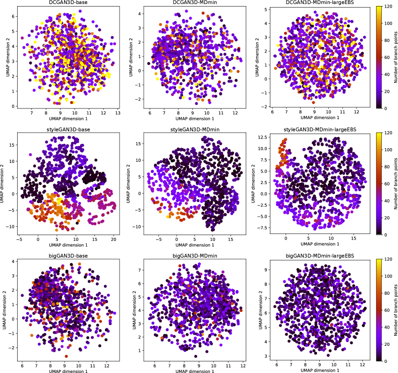
Finally, the relationship between the latent space and the distribution of branch points was investigated using the UMAP dimensionality reduction technique (McInnes et al., 2020). Using the freely available implementation of UMAP444https://umap-learn.readthedocs.io/en/latest/index.html, accessed Oct 2021, the 512-dimensional latent spaces for each method ( for DCGAN3D and bigGAN3D, for styleGAN3D) were transformed into a two-dimensional embedded space. The embedded space was calculated using 50000 random samples to mediate the curse of dimensionality. For 1000 of these samples, the original latent vectors were passed through the corresponding GAN model to produce fake images which could then be analysed as above to find the number of branch points. Latent space structure could then be visualised by labelling each point in the embedded latent space with its corresponding number of branch points.
4 Results
4.1 Model Selection
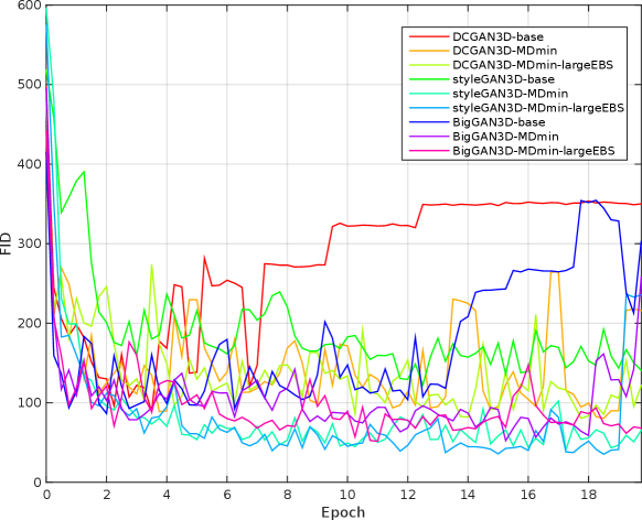
Table 3 shows the minimum observed FIDs for each model, as well as the average and standard deviation (SD) of the minimum over multiple runs. The SD of the minimum FID over the five runs provides a measure of training stability, since it reflects the ability of the method to provide similar results under different initialisations and sequences of training images. The significance of the effects of the MDmin and larger effective batch size techniques was established by performing Welch’s -test on the minimum FID in the five training runs for pairs of methods using the same generator architecture (Figure 4). FID values and network losses throughout the training are provided in Appendix E.
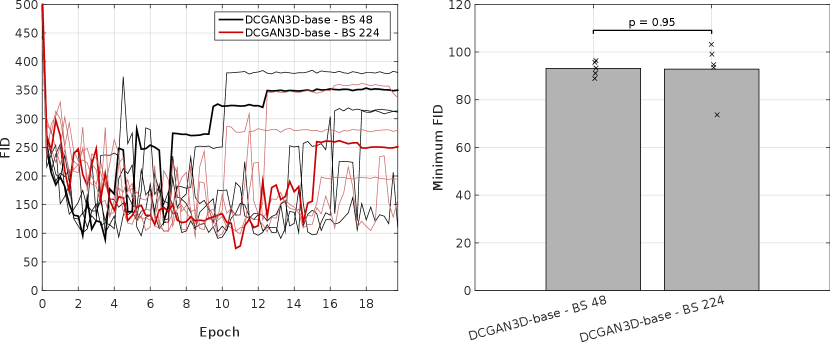
For the DCGAN3D method, including the MDmin layer provides a small, non-significant () improvement, reducing the minimum FID from to and the average minimum FID only from to . The increased SD over five runs suggests that the modest performance improvement comes at the cost of reduced training stability. In addition, we found that the performance of DCGAN3D-base was not significantly affected by batch size (Appendix E).
On the other hand, MDmin was observed to have a significant effect for the styleGAN3D architecture. Without the MDmin layer, the minimum FID observed was , with an average minimum of . Including the MDmin layer reduced this to a minimum of with an average of (); a reduction in both mean and SD representing improved training stability. For the bigGAN3D architecture, the use of MDmin reduced FID from to which was a significant improvement ().
The heuristic method to increase the effective batch size (largeEBS) provided non-significant improvements for the DCGAN3D and bigGAN3D architectures, although for the styleGAN3D architecture, the minimum FID reduced from with just the MDmin layer to when using the increased effective batch size, reflecting a significant reduction in mean minimum FID ().
| Minimum FID | Average minimum FID over five runs | |
|---|---|---|
| DCGAN3D-base | 89.0 | 93.13.1 |
| DCGAN3D-MDmin | 80.3 | 91.09.0 |
| DCGAN3D-MDmin-largeEBS | 80.5 | 86.85.1 |
| styleGAN3D-base | 122.3 | 136.910.7 |
| styleGAN3D-MDmin | 41.0 | 44.84.2 |
| styleGAN3D-MDmin-largeEBS | 35.3 | 38.54.3 |
| bigGAN-base | 86.5 | 93.85.4 |
| bigGAN-MDmin | 52.4 | 58.45.8 |
| bigGAN-MDmin-largeEBS | 51.6 | 57.46.3 |
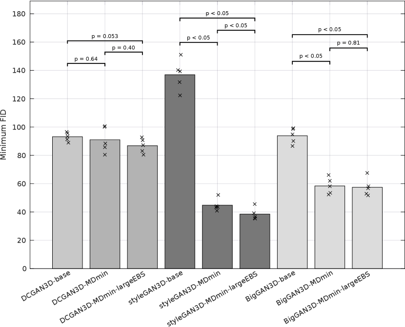
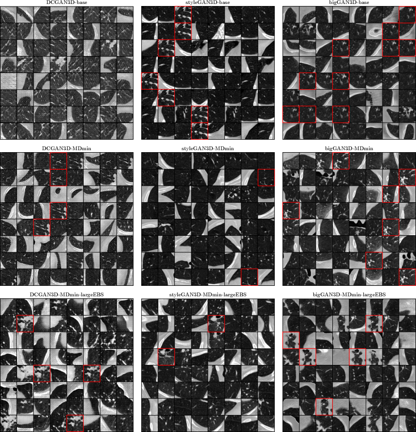
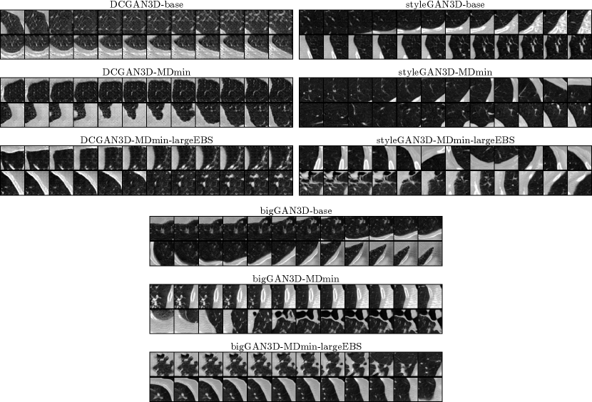
Figure 5 shows some samples for the minimum FID models for each of the GAN methods. The DCGAN3D-base method shows a variety of images, but the image quality is poor, with periodic artefacts visible. On the other hand, the styleGAN3D-base and bigGAN3D-base methods produce high-quality images, but with severe mode collapse. The DCGAN3D-MDmin and DCGAN3D-MDmin-largeEBS methods improve on image quality compared to DCGAN3D-base, but some mode collapse has arisen. This seems to contradict the purpose of the MDmin and largeEBS techniques, though it should be noted that the minimum FID for the best DCGAN3D-base training run occurred early in training, whereas the DCGAN3D-MDmin method reached a minimum at a later point. Because of this, a direct comparison of the variability of the two methods is not appropriate, since mode collapse usually occurs later in training.
In contrast to DCGAN3D, the styleGAN3D-MDmin model reduces mode collapse while retaining image quality compared to the styleGAN-base method. For bigGAN3D, the MDmin did not visibly reduce mode collapse to the same extent as for styleGAN, despite the significant drop in FID recorded in Table 3. However, image quality seems to be qualitatively improved, with more structure visible within the lung parenchyma. Similarly to the DCGAN3D methods, this is likely due to the early occurrence of the minimum FID for the bigGAN3D-base method, before image quality was stable. Using the largeEBS trick seems to further reduce mode collapse for the styleGAN architecture, whereas for the bigGAN3D architecture the effect was negligible.
Finally, Figure 6 shows interpolations between two randomly sampled latent codes for each of the minimum FID models. Note that DCGAN3D and bigGAN3D methods were spherically interpolated in -space, whereas styleGAN methods were linearly interpolated in -space, as described in the original description of the method (Karras et al., 2019). A smooth latent space is a desirable quality of GAN models, which should be reflected by smooth transitions between sampled images. The DCGAN3D methods provide smooth transitions despite their poor image quality. The bigGAN3D methods also exhibit smoothness, with a superior image quality. In general the styleGAN3D interpolations in -space are smooth, although some discontinuities/non-smooth regions are present, possibly due to interpolations traversing low-density regions of -space.
4.2 Observer Study
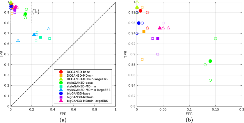
Figure 7 shows the results of the observer study. The DCGAN3D methods, suffering from periodic artefacts and poor image quality, were easily distinguishable from the real images, with and for all models. Slightly improved performance was observed using the bigGAN3D models, with and for the bigGAN3D-MDmin method, but some remaining convolution artefacts made the fake images conspicious compared to real samples. The styleGAN3D-base method performed better than all the DCGAN3D and bigGAN methods, but the mean observer performance was still high at and . When including the MDmin layer, observer performance dropped to and , representing improved model performance. The large effective batch size heuristic worsened styleGAN3D performance slightly, yielding .
4.3 3D Analysis
The FID3D score for each of the models is shown in Table 4. Similarly to the conventional 2D FID scores in Table 3, the best performing method overall is the styleGAN3D-MDmin-largeEBS model which produced a value of 0.57 for the FID3D metric. Interestingly, the effect of the largeEBS method is different in 2D FID compared to 3D FID. For example, the largeEBS reduces 2D FID for the bigGAN3D, compared to using MDmin alone, whereas in terms of FID3D, it rises considerably. We hypothesise that this is because the bigGAN3D architecture has fewer trainable parameters, which means that the MDmin method alone may be fully utilising network capacity. Pushing further with the largeEBS method may cause the training to become more unstable, resulting in worse 3D structure. We leave a full comparison of 2D and 3D FID metrics for future work.
| FID3D | |
|---|---|
| DCGAN3D-base | 4.40 |
| DCGAN3D-MDmin | 4.40 |
| DCGAN3D-MDmin-largeEBS | 1.30 |
| styleGAN3D-base | 3.97 |
| styleGAN3D-MDmin | 2.90 |
| styleGAN3D-MDmin-largeEBS | 0.57 |
| bigGAN3D-base | 4.24 |
| bigGAN3D-MDmin | 1.88 |
| bigGAN3D-MDmin-largeEBS | 6.05 |
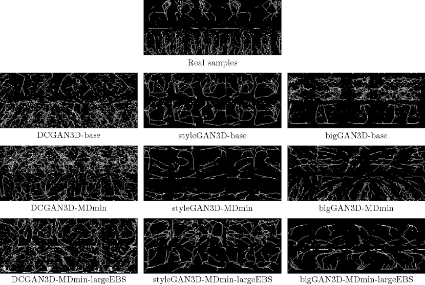
Figure 8 shows some example skeletons calculated from random outputs of each GAN model. The DCGAN3D models provide noisy skeleton images, due to the poor quality of the generated samples. In contrast the styleGAN3D and bigGAN3D outputs produce cleaner skeletons with clearer structure, more closely resembling real images.
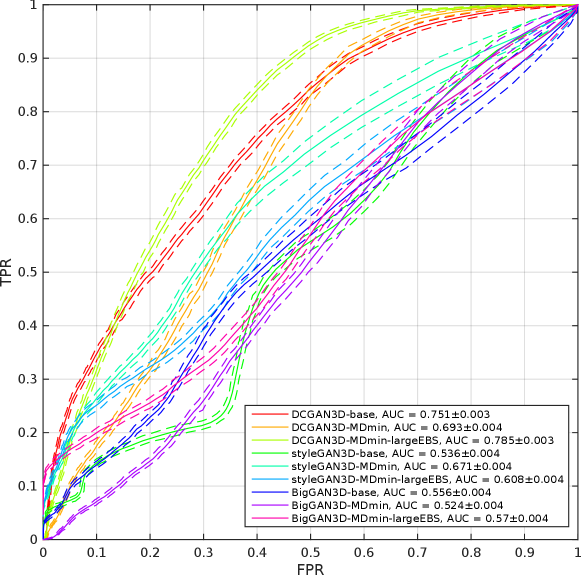
To analyse the distributions of 3D branch points in real and fake images, ROC curves were produced for each method by varying a threshold number of branch points and recording the true and false positive rates (TPR and FPR) of the resulting binary classification. Methods that generate fake images with a similar distribution of branch points to the real data will produce areas under the ROC curve (AUCs) closer to 0.5, and vice versa. Figure 9 shows the ROC curves each of the methods. The DCGAN methods provide AUCs of (DCGAN-base), (DCGAN3D-MDmin), and (DCGAN3D-MDmin-largeEBS), demonstrating that the DCGAN architecture is unable to produce a realistic distribution of branch points. In contrast, the styleGAN3D architecture produces distributions of branch points closer to the real one, reflected by AUC values of for styleGAN3D-base, for styleGAN3D-MDmin, and for styleGAN3D-MDmin-largeEBS. Overall, the bigGAN3D methods provided the best performance, with a lowest AUC of .
The UMAP visualisation of the latent spaces, and their relationship to the number of branch points are shown in Figure 10. For the DCGAN3D and bigGAN3D methods, the UMAP-embedded space shows no structure since the -space is by design distributed normally. Furthermore, no correspondence is apparent between the position of a point in the embedded space and the number of branch points in the corresponding generated image. Conversely, the styleGAN3D methods show both structure in the shape of the -space, and a correspondence between position and number of branch points. This suggests that higher level concepts are contributing to the structure of the full latent space, agreeing with previous literature on the use of styleGAN for medical image generation (Quiros et al., 2021). This is an interesting result, opening the possibility for further investigation into the structure of the latent space with respect to other semantically meaningful features in future work.
It is also important to emphasise that the lack of correspondence between UMAP embeddings and the number of branch points for the bigGAN3D and DCGAN3D methods does not suggest that the full -dimensional latent spaces for these methods are not ordered with respect to the number of branch points, just that any such correspondence is not preserved under the UMAP transformation. Additional analysis to explore whether such correspondence exists for the DCGAN3D and bigGAN3D methods remains for future work.
5 Discussion
The aim of this work was to investigate the applicability and transferability of existing 2D GAN models for the problem of generating 3D patches to model the appearance of healthy lung tissue in pulmonary CT images. Although there has been much research using GANs to generate images of pulmonary nodules (Liu et al., 2018; Jin et al., 2018; Xu et al., 2019; Yang et al., 2019; Bu et al., 2021; Suh et al., 2021; Wang et al., 2021), we believe we are the first to take the next step to specifically model healthy lung tissue.
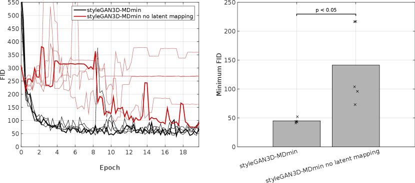
Three architectures were selected from the literature: DCGAN, styleGAN and bigGAN. Results show that the three methods have very different characteristic behaviour. From a visual inspection of generated images, the DCGAN3D-base model was capable of generating a higher variety of images than the styleGAN3D and bigGAN networks (Figure 5), but at the cost of reduced image quality reflected by poor performance in a human observer study (Figure 7) and a higher FID (Table 3 and Figure 4). In contrast, the styleGAN3D-base architecture produced more realistic images that performed better in the observer study and had a more realistic 3D structure (Figures 8 and 9), but at the cost of severe mode collapse that required a minibatch discrimination (MDmin) layer to mitigate. In terms of the FID metric the styleGAN3D methods with MDmin performed best even taking into account remaining mode collapse (Table 3 and Figure 4). Use of the latent mapping network was crucial to the performance of the styleGAN3D methods: omitting it caused training to become unstable and greatly increased the minimum FID (Appendix E).
Despite the strong performance of the styleGAN3D methods in terms of FID and a human observer study, the bigGAN methods were best at learning the distribution of a semantically meaningful quantity (Figure 9), even with a smaller number of trainable parameters ( million for bigGAN3D vs million for styleGAN3D). These results suggest a number of possible improvements to be made in future work: 1) training a bigGAN3D with the same number of parameters as styleGAN3D may lead to better performance in the other metrics while maintaining the distribution of semantically important features, and 2) combining components from styleGAN3D and bigGAN3D architectures, for example by upgrading the bigGAN architecture to allow style-based generation, could yield a method superior in all metrics.
Beyond the networks and architectural components investigated in this work, many more possibilities remain, including the exploration of upgraded styleGAN approaches (Karras et al., 2020, 2021) and autoencoder models such as the high-quality VQ-VAE family (van den Oord et al., 2017; Razavi et al., 2019). The methodology and results presented here represent an important baseline for such future investigations.
Another area for future research is the inclusion of positional information in the GAN models. Currently, our models treat the generation task in a ‘bag-of-patches’ fashion, i.e. ignoring the potentially important spatial context for each patch. By including positional information such as in Lin et al. (2019); Dosovitskiy et al. (2021), the models could be trained to learn the distribution of healthy tissue appearance at each position within the lung, utilising the prior information to help training. However, these methods would need a greater amount of training data, and would take longer to train.
In any case the use of patch-based generators as investigated in this work may hinder application of such methods to a downstream task. Although the query image can be decomposed into patches and then passed through the anomaly detection/reconstruction pipeline, ensuring continuity/consistency between the overlapping output patches may be difficult. In theory a GAN that has learnt the full data distribution should be shift-invariant (given that translated patches remain valid patches), but sub-optimal GAN models are likely to suffer artefacts that would need addressing in future work.
A potential solution to this issue would be to perform whole-volume image generation, completely obviating the need to work with patches. While there has been recent research into modelling large 3D volumes with GANs (Uzunova et al., 2020; Sun et al., 2020; Pesaranghader et al., 2021; Hong et al., 2021), the modelling of entire 3D volumes will require a much larger amount of data in order to fully model the data distribution. The use of smaller datasets has been shown to yield whole-lung GAN models suitable for a data augmentation task (Pesaranghader et al., 2021), but there is currently insufficient evidence that the models capture well the data distribution everywhere, as would be required for an anomaly detection or image reconstruction task. Nonetheless, these models can be evaluated under the pipeline introduced in this work by firstly generating a number of whole-volume images, and then breaking these into patches for subsequent analysis.
6 Conclusions
GAN models are of interest in anomaly detection and image reconstruction tasks in a variety of medical imaging applications. However, due to variations in the underlying structure of datasets, GAN models must be re-adapted, re-trained, and re-assessed for each new application, which is a non-trivial task.
In this work we adapted three GAN models from the natural image literature to the task of 3D healthy lung CT patch generation, and evaluated their performances. Of the three architectures investigated, the styleGAN3D approaches provided the best performance according to FID values and observer studies, while the bigGAN3D architecture was superior in an analysis of 3D structure. The use of minibatch discrimination was shown to be crucial for the styleGAN3D architecture in order to avoid excessive mode collapse and inclusion of a latent mapping network was shown to allow styleGAN3D to produce a latent space with semantic meaning. However, despite the promising results, we conclude that none of the investigated methods are currently suitable for the downstream tasks of anomaly detection or image reconstruction. Future directions of research are proposed, including the use of positional encoding or whole-volume generation, to further improve on these results. Overall, the results and analyses presented in this work provide an important baseline for future research into the use of generative models in 3D healthy lung CT patch modelling.
Acknowledgments
This work was funded by the EPSRC grant [EP/P023509/1] and supported by funding from the Wellcome/EPSRC Centre for Medical Engineering [WT203148/Z/16/Z]; the National Institute for Health Research (NIHR) Biomedical Research Centre based at Guy’s and St Thomas’ NHS Foundation Trust and King’s College London; and the UKRI London Medical Imaging and Artificial Intelligence Centre for Value Based Healthcare.
Ethical Standards
The work follows appropriate ethical standards in conducting research and writing the manuscript, following all applicable laws and regulations regarding treatment of animals or human subjects.
Conflicts of Interest
There are no conflicts of interest to declare.
References
- Arjovsky et al. (2017) Martin Arjovsky, Soumith Chintala, and Léon Bottou. Wasserstein Generative Adversarial Networks. In Doina Precup and Yee Whye Teh, editors, Proc. 34th Int. Conf. Mach. Learn., volume 70 of Proceedings of Machine Learning Research, pages 214–223. PMLR, 2017.
- Barile et al. (2021) Berardino Barile, Aldo Marzullo, Claudio Stamile, Françoise Durand-Dubief, and Dominique Sappey-Marinier. Data augmentation using generative adversarial neural networks on brain structural connectivity in multiple sclerosis. Comput. Methods Programs Biomed., 206:106113, 2021.
- Brock et al. (2019) Andrew Brock, Jeff Donahue, and Karen Simonyan. Large scale GAN training for high fidelity natural image synthesis. In 7th Int. Conf. Learn. Represent. ICLR 2019, 2019.
- Bu et al. (2021) Tian Bu, Zhiyong Yang, Shan Jiang, Guobin Zhang, Hongyun Zhang, and Lin Wei. 3D conditional generative adversarial network-based synthetic medical image augmentation for lung nodule detection. Int. J. Imaging Syst. Technol., 31(2):670–681, 2021.
- Chen et al. (2019) Sihong Chen, Kai Ma, and Yefeng Zheng. Med3D: Transfer Learning for 3D Medical Image Analysis, 2019. URL https://arxiv.org/abs/1904.00625.
- Dong et al. (2019) Xue Dong, Yang Lei, Tonghe Wang, Matthew Thomas, Leonardo Tang, Walter J Curran, Tian Liu, and Xiaofeng Yang. Automatic multiorgan segmentation in thorax CT images using U-net-GAN. Med. Phys., 46(5):2157–2168, 2019.
- Dosovitskiy et al. (2021) Alexey Dosovitskiy, Lucas Beyer, Alexander Kolesnikov, Dirk Weissenborn, Xiaohua Zhai, Thomas Unterthiner, Mostafa Dehghani, Matthias Minderer, Georg Heigold, Sylvain Gelly, Jakob Uszkoreit, and Neil Houlsby. An Image is Worth 16x16 Words: Transformers for Image Recognition at Scale. In International Conference on Learning Representations, 2021.
- Emami et al. (2018) Hajar Emami, Ming Dong, Siamak P Nejad-Davarani, and Carri K Glide-Hurst. Generating synthetic CTs from magnetic resonance images using generative adversarial networks. Med. Phys., 45(8):3627–3636, 2018.
- Frid-Adar et al. (2018) Maayan Frid-Adar, Idit Diamant, Eyal Klang, Michal Amitai, Jacob Goldberger, and Hayit Greenspan. GAN-based synthetic medical image augmentation for increased CNN performance in liver lesion classification. Neurocomputing, 321:321–331, 2018.
- Goodfellow et al. (2014) Ian Goodfellow, Jean Pouget-Abadie, Mehdi Mirza, Bing Xu, David Warde-Farley, Sherjil Ozair, Aaron Courville, and Yoshua Bengio. Generative Adversarial Nets. In Z Ghahramani, M Welling, C Cortes, N Lawrence, and K Q Weinberger, editors, Adv. Neural Inf. Process. Syst., volume 27. Curran Associates, Inc., 2014.
- Gulrajani et al. (2017) Ishaan Gulrajani, Faruk Ahmed, Martin Arjovsky, Vincent Dumoulin, and Aaron C Courville. Improved Training of Wasserstein GANs. In I Guyon, U V Luxburg, S Bengio, H Wallach, R Fergus, S Vishwanathan, and R Garnett, editors, Adv. Neural Inf. Process. Syst., volume 30. Curran Associates, Inc., 2017.
- Heusel et al. (2017) Martin Heusel, Hubert Ramsauer, Thomas Unterthiner, Bernhard Nessler, and Sepp Hochreiter. GANs Trained by a Two Time-Scale Update Rule Converge to a Local Nash Equilibrium. In I Guyon, U V Luxburg, S Bengio, H Wallach, R Fergus, S Vishwanathan, and R Garnett, editors, Adv. Neural Inf. Process. Syst., volume 30. Curran Associates, Inc., 2017.
- Hong et al. (2021) Sungmin Hong, Razvan Marinescu, Adrian V. Dalca, Anna K. Bonkhoff, Martin Bretzner, Natalia S. Rost, and Polina Golland. 3D-StyleGAN: A Style-Based Generative Adversarial Network for Generative Modeling of Three-Dimensional Medical Images. In Sandy Engelhardt, Ilkay Oksuz, Dajiang Zhu, Yixuan Yuan, Anirban Mukhopadhyay, Nicholas Heller, Sharon Xiaolei Huang, Hien Nguyen, Raphael Sznitman, and Yuan Xue, editors, Deep Generative Models, and Data Augmentation, Labelling, and Imperfections, pages 24–34, Cham, 2021. Springer International Publishing.
- Huang and Belongie (2017) Xun Huang and Serge Belongie. Arbitrary Style Transfer in Real-time with Adaptive Instance Normalization. In Proceedings of the International Conference on Computer Vision (ICCV), volume 2017-Octob, pages 1510–1519. Institute of Electrical and Electronics Engineers Inc., 2017.
- Ioffe and Szegedy (2015) Sergey Ioffe and Christian Szegedy. Batch Normalization: Accelerating Deep Network Training by Reducing Internal Covariate Shift. In Francis Bach and David Blei, editors, Proc. 32nd Int. Conf. Mach. Learn., volume 37 of Proceedings of Machine Learning Research, pages 448–456, Lille, France, 2015. PMLR.
- Isola et al. (2017) Phillip Isola, Jun-Yan Zhu, Tinghui Zhou, and Alexei A. Efros. Image-to-image translation with conditional adversarial networks. In Proceedings of the IEEE Conference on Computer Vision and Pattern Recognition (CVPR), 2017.
- Jin et al. (2018) Dakai Jin, Ziyue Xu, Youbao Tang, Adam P. Harrison, and Daniel J. Mollura. CT-Realistic Lung Nodule Simulation from 3D Conditional Generative Adversarial Networks for Robust Lung Segmentation. In Alejandro F. Frangi, Julia A. Schnabel, Christos Davatzikos, Carlos Alberola-López, and Gabor Fichtinger, editors, Medical Image Computing and Computer Assisted Intervention – MICCAI 2018, pages 732–740, Cham, 2018. Springer International Publishing.
- Jolicoeur-Martineau (2019) Alexia Jolicoeur-Martineau. The relativistic discriminator: a key element missing from standard GAN. In International Conference on Learning Representations, 2019. URL https://openreview.net/forum?id=S1erHoR5t7.
- Karras et al. (2018) Tero Karras, Timo Aila, Samuli Laine, and Jaakko Lehtinen. Progressive growing of GANs for improved quality, stability, and variation. In 6th Int. Conf. Learn. Represent. ICLR 2018 - Conf. Track Proc., 2018.
- Karras et al. (2019) Tero Karras, Samuli Laine, and Timo Aila. A style-based generator architecture for generative adversarial networks. In Proc. IEEE Comput. Soc. Conf. Comput. Vis. Pattern Recognit., volume 2019-June, pages 4396–4405, 2019.
- Karras et al. (2020) Tero Karras, Samuli Laine, Miika Aittala, Janne Hellsten, Jaakko Lehtinen, and Timo Aila. Analyzing and Improving the Image Quality of StyleGAN. In Proceedings of the IEEE Conference on Computer Vision and Pattern Recognition (CVPR), pages 8107–8116, 2020.
- Karras et al. (2021) Tero Karras, Miika Aittala, Samuli Laine, Erik Härkönen, Janne Hellsten, Jaakko Lehtinen, and Timo Aila. Alias-Free Generative Adversarial Networks. In M. Ranzato, A. Beygelzimer, Y. Dauphin, P.S. Liang, and J. Wortman Vaughan, editors, Advances in Neural Information Processing Systems, volume 34, pages 852–863. Curran Associates, Inc., 2021.
- Kingma and Ba (2015) Diederik P. Kingma and Jimmy Lei Ba. Adam: A method for stochastic optimization. In 3rd Int. Conf. Learn. Represent. ICLR 2015 - Conf. Track Proc., 2015.
- Lample et al. (2017) Guillaume Lample, Neil Zeghidour, Nicolas Usunier, Antoine Bordes, Ludovic DENOYER, and Marc' Aurelio Ranzato. Fader Networks: Manipulating Images by Sliding Attributes. In I. Guyon, U. V. Luxburg, S. Bengio, H. Wallach, R. Fergus, S. Vishwanathan, and R. Garnett, editors, Advances in Neural Information Processing Systems, volume 30. Curran Associates, Inc., 2017.
- Lim and Ye (2017) Jae Hyun Lim and Jong Chul Ye. Geometric GAN. arXiv, page 1705.02894, 2017.
- Lin et al. (2019) Chieh Hubert Lin, Chia-Che Chang, Yu-Sheng Chen, Da-Cheng Juan, Wei Wei, and Hwann-Tzong Chen. COCO-GAN: Generation by Parts via Conditional Coordinating. In Proceedings of the International Conference on Computer Vision (ICCV), 2019.
- Liu et al. (2018) Siqi Liu, Eli Gibson, Sasa Grbic, Zhoubing Xu, Arnaud Arindra Adiyoso Setio, Jie Yang, Bogdan Georgescu, and Dorin Comaniciu. Decompose to manipulate: Manipulable Object Synthesis in 3D Medical Images with Structured Image Decomposition. arXiv, page 1812.01737, 2018.
- Mao et al. (2017) Xudong Mao, Qing Li, Haoran Xie, Raymond Y K Lau, Zhen Wang, and Stephen Paul Smolley. Least Squares Generative Adversarial Networks. In Proceedings of the International Conference on Computer Vision (ICCV), pages 2813–2821, 2017.
- McInnes et al. (2020) Leland McInnes, John Healy, and James Melville. UMAP: Uniform Manifold Approximation and Projection for Dimension Reduction. arXiv, page 1802.03426, 2020.
- Miyato et al. (2018) Takeru Miyato, Toshiki Kataoka, Masanori Koyama, and Yuichi Yoshida. Spectral normalization for generative adversarial networks. In 6th Int. Conf. Learn. Represent. ICLR 2018 - Conf. Track Proc., 2018.
- Montalt-Tordera et al. (2021) Javier Montalt-Tordera, Vivek Muthurangu, Andreas Hauptmann, and Jennifer Anne Steeden. Machine learning in Magnetic Resonance Imaging: Image reconstruction. Phys. Medica, 83:79–87, 2021.
- Perarnau et al. (2016) Guim Perarnau, Joost van de Weijer, Bogdan Raducanu, and Jose M Álvarez. Invertible Conditional GANs for image editing. arXiv, page 1611.06355, 2016.
- Pesaranghader et al. (2021) Ahmad Pesaranghader, Yiping Wang, and Mohammad Havaei. CT-SGAN: Computed Tomography Synthesis GAN. In Sandy Engelhardt, Ilkay Oksuz, Dajiang Zhu, Yixuan Yuan, Anirban Mukhopadhyay, Nicholas Heller, Sharon Xiaolei Huang, Hien Nguyen, Raphael Sznitman, and Yuan Xue, editors, Deep Generative Models, and Data Augmentation, Labelling, and Imperfections, pages 67–79, Cham, 2021. Springer International Publishing.
- Quiros et al. (2021) Adalberto Claudio Quiros, Roderick Murray-Smith, and Ke Yuan. PathologyGAN: Learning deep representations of cancer tissue. Machine Learning for Biomedical Imaging, 1, 2021.
- Radford et al. (2016) Alec Radford, Luke Metz, and Soumith Chintala. Unsupervised representation learning with deep convolutional generative adversarial networks. In 4th Int. Conf. Learn. Represent. ICLR 2016 - Conf. Track Proc. International Conference on Learning Representations, ICLR, 2016.
- Ravishankar et al. (2020) Saiprasad Ravishankar, Jong Chul Ye, and Jeffrey A Fessler. Image Reconstruction: From Sparsity to Data-Adaptive Methods and Machine Learning. Proc. IEEE, 108(1):86–109, 2020.
- Razavi et al. (2019) Ali Razavi, Aaron van den Oord, and Oriol Vinyals. Generating diverse high-fidelity images with vq-vae-2. In H. Wallach, H. Larochelle, A. Beygelzimer, F. d'Alché-Buc, E. Fox, and R. Garnett, editors, Advances in Neural Information Processing Systems, volume 32. Curran Associates, Inc., 2019. URL https://proceedings.neurips.cc/paper/2019/file/5f8e2fa1718d1bbcadf1cd9c7a54fb8c-Paper.pdf.
- Reader et al. (2020) Andrew J. Reader, Guillaume Corda, Abolfazl Mehranian, Casper da Costa-Luis, Sam Ellis, and Julia A. Schnabel. Deep Learning for PET Image Reconstruction. IEEE Trans. Radiat. Plasma Med. Sci., 5(1):1–25, 2020.
- Salimans et al. (2016) Tim Salimans, Ian Goodfellow, Wojciech Zaremba, Vicki Cheung, Alec Radford, and Xi Chen. Improved Techniques for Training GANs. arXiv, page 1606.03498v1, 2016.
- Schlegl et al. (2019) Thomas Schlegl, Philipp Seeböck, Sebastian M. Waldstein, Georg Langs, and Ursula Schmidt-Erfurth. f-AnoGAN: Fast unsupervised anomaly detection with generative adversarial networks. Med. Image Anal., 54:30–44, 2019.
- Setio et al. (2017) Arnaud Arindra Adiyoso Setio, Alberto Traverso, Thomas de Bel, Moira S.N. Berens, Cas van den Bogaard, Piergiorgio Cerello, Hao Chen, Qi Dou, Maria Evelina Fantacci, Bram Geurts, Robbert van der Gugten, Pheng Ann Heng, Bart Jansen, Michael M.J. de Kaste, Valentin Kotov, Jack Yu-Hung Lin, Jeroen T.M.C. Manders, Alexander Sóñora Mengana, Juan Carlos García-Naranjo, Evgenia Papavasileiou, Mathias Prokop, Marco Saletta, Cornelia M Schaefer-Prokop, Ernst T. Scholten, Luuk Scholten, Miranda M. Snoeren, Ernesto Lopez Torres, Jef Vandemeulebroucke, Nicole Walasek, Guido C.A. Zuidhof, Bram van Ginneken, and Colin Jacobs. Validation, comparison, and combination of algorithms for automatic detection of pulmonary nodules in computed tomography images: The LUNA16 challenge. Med. Image Anal., 42:1–13, 2017.
- Sinha et al. (2020) Samarth Sinha, Zhengli Zhao, Anirudh Goyal, Colin Raffel, and Augustus Odena. Top-k Training of GANs: Improving GAN Performance by Throwing Away Bad Samples. In H. Larochelle, M. Ranzato, R. Hadsell, M. F. Balcan, and H. Lin, editors, Advances in Neural Information Processing Systems, volume 33, pages 14638–14649. Curran Associates, Inc., 2020.
- Suh et al. (2021) Sungho Suh, Sojeong Cheon, Dong-Jin Chang, Deukhee Lee, and Yong Oh Lee. Sequential Lung Nodule Synthesis Using Attribute-Guided Generative Adversarial Networks. In Marleen de Bruijne, Philippe C. Cattin, Stéphane Cotin, Nicolas Padoy, Stefanie Speidel, Yefeng Zheng, and Caroline Essert, editors, Medical Image Computing and Computer Assisted Intervention – MICCAI 2021, pages 402–411, Cham, 2021. Springer International Publishing.
- Sun et al. (2020) Li Sun, Junxiang Chen, Yanwu Xu, Mingming Gong, Ke Yu, and Kayhan Batmanghelich. Hierarchical Amortized Training for Memory-efficient High Resolution 3D GAN . In MedNeurIPS 2020, 2020.
- Uzunova et al. (2020) Hristina Uzunova, Jan Ehrhardt, and Heinz Handels. Memory-efficient GAN-based domain translation of high resolution 3D medical images. Computerized Medical Imaging and Graphics, 86:101801, 2020.
- van den Oord et al. (2017) Aaron van den Oord, Oriol Vinyals, and Koray Kavukcuoglu. Neural discrete representation learning. In I. Guyon, U. Von Luxburg, S. Bengio, H. Wallach, R. Fergus, S. Vishwanathan, and R. Garnett, editors, Advances in Neural Information Processing Systems, volume 30. Curran Associates, Inc., 2017. URL https://proceedings.neurips.cc/paper/2017/file/7a98af17e63a0ac09ce2e96d03992fbc-Paper.pdf.
- Wang et al. (2021) Qiuli Wang, Xiaohong Zhang, Wei Zhang, Mingchen Gao, Sheng Huang, Jian Wang, Jiuquan Zhang, Dan Yang, and Chen Liu. Realistic Lung Nodule Synthesis With Multi-Target Co-Guided Adversarial Mechanism. IEEE Transactions on Medical Imaging, 40(9):2343–2353, 2021.
- Xu et al. (2019) Ziyue Xu, Xiaosong Wang, Hoo-Chang Shin, Holger Roth, Dong Yang, Fausto Milletari, Ling Zhang, and Daguang Xu. Tunable CT Lung Nodule Synthesis Conditioned on Background Image and Semantic Features. In Ninon Burgos, Ali Gooya, and David Svoboda, editors, Simulation and Synthesis in Medical Imaging, pages 62–70, Cham, 2019. Springer International Publishing.
- Yang et al. (2019) Jie Yang, Siqi Liu, Sasa Grbic, Arnaud Arindra Adiyoso Setio, Zhoubing Xu, Eli Gibson, Guillaume Chabin, Bogdan Georgescu, Andrew F. Laine, and Dorin Comaniciu. Class-Aware Adversarial Lung Nodule Synthesis In CT Images. In 2019 IEEE 16th International Symposium on Biomedical Imaging (ISBI 2019), pages 1348–1352, 2019.
- Yi et al. (2019) Xin Yi, Ekta Walia, and Paul Babyn. Generative adversarial network in medical imaging: A review. Med. Image Anal., 58:101552, 2019.
- Zhang et al. (2019) Han Zhang, Ian Goodfellow, Dimitris Metaxas, and Augustus Odena. Self-Attention Generative Adversarial Networks. In Kamalika Chaudhuri and Ruslan Salakhutdinov, editors, Proceedings of the 36th International Conference on Machine Learning, volume 97 of Proceedings of Machine Learning Research, pages 7354–7363. PMLR, 2019.
- Zhu et al. (2017) Jun Yan Zhu, Taesung Park, Phillip Isola, and Alexei A. Efros. Unpaired Image-to-Image Translation Using Cycle-Consistent Adversarial Networks. In Proceedings of the International Conference on Computer Vision (ICCV), volume 2017-Octob, pages 2242–2251, 2017.
A DCGAN3D generator architecture
| DCGAN3D generator |
|---|
| Input: |
| ConvTranspose3d , stride 1, pad 0, no bias, 512512 |
| BatchNorm3d + ReLU |
| ConvTranspose3d , stride 2, pad , no bias, 512256 |
| BatchNorm3d + ReLU |
| ConvTranspose3d , stride 2, pad 1, no bias, 256128 |
| BatchNorm3d + ReLU |
| ConvTranspose3d , stride 2, pad 1, no bias, 12864 |
| BatchNorm3d + ReLU |
| ConvTranspose3d , stride 2, pad 1, no bias, 641 |
| Tanh |
| Output: |
B styleGAN3D generator architecture
| styleGAN3D generator: latent mapping network |
|---|
| Input: |
| FC, 512 512 |
| Leaky ReLU 0.2 |
| FC, 512 512 |
| Leaky ReLU 0.2 |
| FC 512 512 |
| Leaky ReLU 0.2 |
| FC, 512 512 |
| Leaky ReLU 0.2 |
| FC, 512 512 |
| Leaky ReLU 0.2 |
| FC, 512 512 |
| Leaky ReLU 0.2 |
| FC, 512 512 |
| Leaky ReLU 0.2 |
| FC, 512 512 |
| Leaky ReLU 0.2 |
| Output: |
| styleGAN3D generator: synthesis network |
|---|
| Input: , |
| AdaIN, Conv3d , stride 1, pad 1, no bias, 512 |
| Leaky ReLU 0.2 |
| AdaIN, nearest-neighbour upsample, Conv3d , stride 1, pad 1, no bias, 512 |
| Leaky ReLU 0.2 |
| AdaIN, Conv3d , stride 1, pad 1, no bias, 256 |
| Leaky ReLU 0.2 |
| AdaIN, nearest-neighbour upsample, Conv3d , stride 1, pad 1, no bias, 256 |
| Leaky ReLU 0.2 |
| AdaIN, Conv3d , stride 1, pad 1, no bias, 128 |
| Leaky ReLU 0.2 |
| AdaIN, nearest-neighbour upsample, Conv3d , stride 1, pad 1, no bias, 128 |
| Leaky ReLU 0.2 |
| AdaIN, Conv3d , stride 1, pad 1, no bias, 64 |
| AdaIN, nearest-neighbour upsample, Conv3d , stride 1, pad 1, no bias, 64 |
| Leaky ReLU 0.2 |
| AdaIN, Conv3d , stride 1, pad 1, no bias, 32 |
| Leaky ReLU 0.2 |
| AdaIN, nearest-neighbour upsample, Conv3d , stride 1, pad 1, no bias, 32 |
| Leaky ReLU 0.2 |
| AdaIN, Conv3d , stride 1, pad 1, no bias, 16 |
| Tanh |
| Output: |
C bigGAN3D generator architecture
| bigeGAN3D generator |
|---|
| Input: |
| SNFC, 512 6144 |
| Reshape |
| BatchNorm3d + ReLU |
| nearest neighbour upsample, SNConv3d , stride 1, pad 1, bias, 96 96 |
| BatchNorm3d + ReLU |
| SNConv3d , stride 1, pad 1, bias, 96 96 |
| SNConv3d , stride 1, pad 0, bias, 96 96 |
| SelfAttention3D |
| BatchNorm3d + ReLU |
| nearest neighbour upsample, SNConv3d , stride 1, pad 1, bias, 96 48 |
| BatchNorm3d + ReLU |
| SNConv3d , stride 1, pad 1, bias, 48 48 |
| SNConv3d , stride 1, pad 0, bias, 48 48 |
| BatchNorm3d + ReLU |
| nearest neighbour upsample, SNConv3d , stride 1, pad 1, bias, 48 24 |
| BatchNorm3d + ReLU |
| SNConv3d , stride 1, pad 1, bias, 24 24 |
| SNConv3d , stride 1, pad 0, bias, 24 24 |
| BatchNorm3d + ReLU |
| nearest neighbour upsample, SNConv3d , stride 1, pad 1, bias, 24 12 |
| BatchNorm3d + ReLU |
| SNConv3d , stride 1, pad 1, bias, 12 12 |
| SNConv3d , stride 1, pad 0, bias, 12 12 |
| BatchNorm3d + ReLU |
| SNConv3d , stride 1, pad 1, bias, 12 1 |
| Tanh |
| Output: |
D Minibatch Discrimination and Increasing the Effective Batch Size
Minibatch Discrimination: MDmin
The following approach to MD was adopted, calculating the L1 distance, , between two images and within a minibatch as:
| (6) |
where denotes the features of the discriminator network after layer with as the input image. In the traditional minibatch discrimination approach (Salimans et al., 2016), these distances (or some transformation of them) are then either summed or averaged over the minibatch to get a per-image score, i.e. , which is used as input for the subsequent discriminator layer.
We note that taking the sum of allows partial mode collapse to occur if one mode is sufficiently far from the rest of the samples. To overcome this, we propose to take instead the minimum within-batch distance for each image, denoted MDmin, as follows: . This represents the maximum similarity between two samples in the minibatch, providing a consistently clearer signal to the discriminator if these images are mode-collapsed. The scalar values per image, , are then expanded to the correct size and appended to the current feature maps, to provide an extra feature to the subsequent layers of the discriminator.
Increased Effective Batch Size: largeEBS
The MDmin layer described above is able to reduce mode collapse by allowing the discriminator to detect when a minibatch contains similar samples, and feed this information back to the generator. However, mode collapse can clearly still occur, as long as similar samples are unlikely to occur within a minibatch. Size the maximum batch size is bounded by computational limitations (GPU memory), this issue cannot be solved completely by simply increasing the batch size.
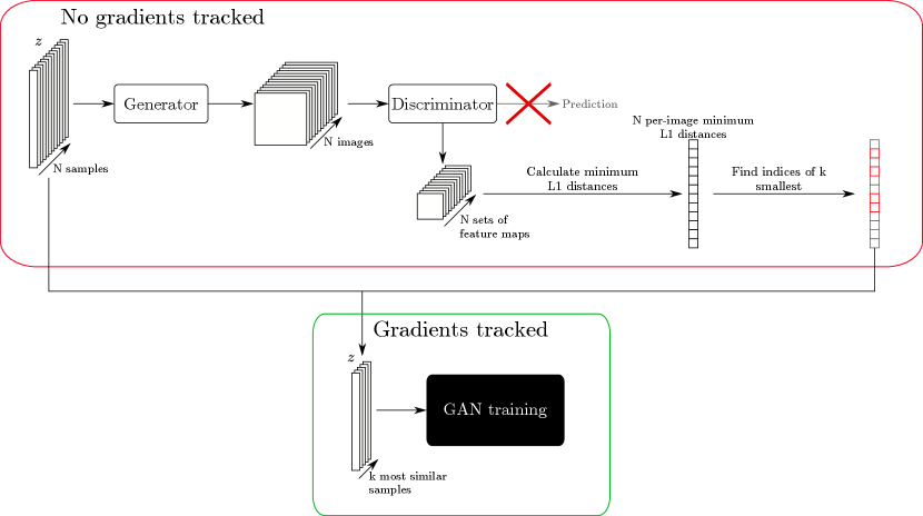
We propose to use a heuristic trick to increase the effective batch size, mitigating the effect described above. First, a large batch of latent codes is sampled and passed through the generator without tracking gradients. This allows a larger batch size than would be normally used in training, since much of the computational load of network training is in the storing of gradients. These generated images are then passed through the discriminator without tracking gradients, and the activation maps at depth are calculated, similarly as for the MDmin layer. The similarity between all pairs of samples is then calculated, as for the MDmin layer, and the minimum for each sample is taken as a measure of how mode-collapsed that particular sample is within the larger minibatch. The most similar images are noted, and the corresponding samples are then used for the subsequent training iteration, ensuring that the networks see the most mode-collapsed samples for training purposes. Figure A1 shows this process schematically. Note that with this method, the upper limit to the effective batch size is no longer dependent on memory, since each pair of images can in theory be loaded to memory as required and do not need to be stored otherwise. Real samples are still selected entirely at random; choosing the most similar samples from a larger batch of real images was seen to degrade performance. Since the learned discriminator representations will not be relevant early in training, we train the networks for epochs as normal before increasing the effective batch size thereafter. Similar heuristic tricks to select the most relevant/useful samples for GAN training are established in the literature, for example in Sinha et al. (2020), although not for the specific case of reducing mode collapse.
E Additional Results