1 Introduction
With the continuous breakthrough of biological microscopic imaging technology, a large number of histopathology images have been produced to assist clinical practice and research. Quantitative, objective, and effective cell analysis based on histopathology images has become an important research direction (Gurcan et al., 2009; Veta et al., 2014). Pathologists usually use information such as the number, density, and distribution of cells in a given area in histopathology images to assess the degree of tissue damage and make a diagnosis (Fusi et al., 2013). Such analysis relies on the detection of the cells of interest. However, manual cell detection performed by pathologists can be time-consuming and error-prone (Wang et al., 2022; van der Laak et al., 2021), especially in areas of high cell density, and automated cell detection methods are needed.
In recent years, deep learning techniques have been successfully applied to various image processing tasks, and they have been increasingly used to analyze histopathology images as well (Lu et al., 2021; Noorbakhsh et al., 2020; Srinidhi et al., 2021; He et al., 2021; van der Laak et al., 2021; Marostica et al., 2021). In particular, convolutional neural networks (CNNs) have been applied to perform automated cell detection in histopathology images. For example, Xu et al. (2016) propose stacked sparse autoencoder for efficient nuclei detection in high-resolution histopathology images of breast cancer; Sirinukunwattana et al. (2016) propose a spatially constrained CNN to perform nuclei detection in routine colon cancer histopathology images. More advanced networks that are originally developed for generic object detection are later used or adapted for cell detection. In these methods, cells of interest are localized by bounding boxes. For example, Cai et al. (2019) have modified Faster R-CNN (Ren et al., 2017) for automatic mitosis detection in breast histopathology images; Sun et al. (2020) use the region proposal network (Ren et al., 2017), Faster R-CNN, and RetinaNet (Lin et al., 2017), as well as their adapted versions that enable similarity learning, for signet ring cell detection in histopathology images.
To train advanced CNN-based cell detection models, usually every cell of interest in the training images should be annotated (e.g., with a bounding box and the identification of its type), and instances in unannotated regions111 Usually large whole-slide images are acquired for histopathology image analysis, and they are cropped into patches for cell annotation or detection. Here, the unannotated regions refer to the regions without annotated cells in image patches that are annotated. are considered negative training samples. However, due to the complexity and large number of cells in histopathology images, completely annotating every cell of interest in the training images can be challenging. It is more practical to perform incomplete annotation, where only a fraction of the cells of interest are annotated and the unannotated areas may also contain positive instances (i.e., cells of interest) (Li et al., 2019). The annotations may even be sparse with only a few annotated cells in a training image to reduce the annotation load (Li et al., 2020). Since the instances in unannotated areas are not necessarily true negative samples when the annotations are incomplete, typical network training procedures designed for complete annotations can be problematic for incomplete annotations and degrade the detection performance.
Li et al. (2020) propose to solve the problem of incomplete annotations for cell detection in histopathology images by calibrating the loss function during network training. Specifically, it is observed that the density of the detection boxes associated with positive instances is much greater than the box density associated with negative instances. Therefore, the Boxes Density Energy (BDE) is developed in Li et al. (2020) to calibrate the loss terms associated with the training samples in unannotated areas, where the samples with higher box density are calibrated to have smaller weights, as they are less likely to be truly negative. It is shown in Li et al. (2020), as well as in its extended journal version Li et al. (2021), that when the annotations are incomplete, the detection performance is improved with the BDE loss calibration compared with the typical training strategy that treats all instances in unannotated areas as negative. To the best of our knowledge, this is the only existing work that addresses the problem of incomplete annotations for cell detection in histopathology images222The work in Li et al. (2019) requires the annotated mask of each instance in addition to the bounding box, and thus it addresses a different problem., and the development of methods that may better solve this problem is still desired.
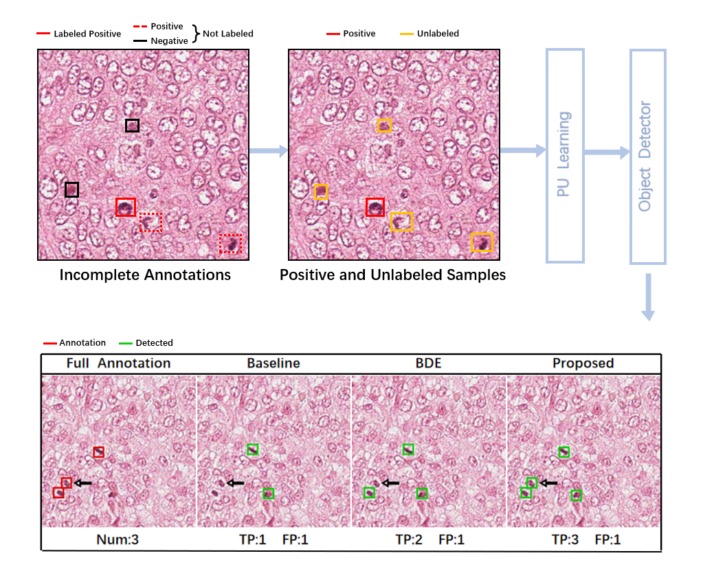
In this work, we continue to explore the problem of incomplete annotations for CNN-based cell detection in histopathology images. Since unannotated areas in incomplete annotations may include both positive and negative samples, i.e., the labels of the instances in these regions are unknown, whereas annotated samples are all positive, we propose to address the problem of incomplete annotations with a positive-unlabeled (PU) learning framework (Elkan and Noto, 2008; Kiryo et al., 2017). We integrate our method with advanced object detectors, where a classification loss and a box regression loss are combined for network training, and reformulate the classification loss with PU learning. Specifically, the classification loss terms associated with negative samples are revised, so that they can be approximated with positively labeled instances and instances with unknown labels. We first derive the approximation for the case of binary cell detection, where only one type of cell is of interest. Then, the approximation is extended to the case of multi-class cell detection, where more than one types of cells are to be identified given incomplete annotations. To evaluate the proposed method, we performed experiments on four publicly available datasets of histopathology images, and for demonstration, Faster R-CNN (Ren et al., 2017) was used as our backbone detection network, as it has previously achieved excellent cell detection results (Sun et al., 2020; Cai et al., 2019). The experimental results on the four datasets show that the proposed method leads to improved cell detection performance given incomplete annotations for training.
This manuscript is an extension of our conference paper (Zhao et al., 2021) presented at MICCAI 2021. In the current manuscript, we have substantially extended our work in terms of both methodology and evaluation. Specifically, we have extended the proposed framework from the binary cell detection problem considered in Zhao et al. (2021) to multi-class cell detection, where the corresponding approximation of loss terms is derived and the strategy of hyperparameter selection is determined; in addition, we have evaluated our method more comprehensively with three additional publicly available datasets under various experimental settings. The code of the proposed method is available at https://github.com/zipeizhao/PU-learning-for-cell-detection.
We organize the remaining of the paper as follows. Section 2 presents the proposed approach to cell detection in histopathology images given incomplete annotations. In Section 3, we describe the cell detection results on the publicly available datasets. Section 4 discusses the results and future works. Finally, Section 5 summarizes the proposed work.
2 Methods
In this section, we first introduce how CNN-based cell detection methods are conventionally trained given completely annotated training data. Then, we present the proposed approach that adapts PU learning to address the problem of incomplete annotations for cell detection in histopathology images. Finally, the implementation details are given.
2.1 Background: cell detection with complete annotations for training
CNN-based methods have greatly improved the performance of object detection. These methods have also been applied to cell detection and have achieved promising results. For a typical modern CNN-based object detector, e.g., Faster R-CNN (Ren et al., 2017), convolutional layers are used to extract feature maps from input images, and the extracted feature maps are then fed into subsequent layers to predict the location and class of the objects of interest. Most commonly, a bounding box333Depending on the object detector, the bounding box can be defined differently. For the commonly used Faster R-CNN, it is produced by the detection network based on each anchor. For a more detailed description of the bounding box and anchor, we refer readers to Ren et al. (2017). is generated to indicate the position of an object of interest, which is produced by the regression head of the detector. For convenience, the predicted position of the bounding box is denoted by , where , , , and represent the coordinate in the horizontal direction, coordinate in the vertical direction, width, and height of the bounding box, respectively. The class of the object is simultaneously predicted by the classification head of the detector, where the likelihood of the instance belonging to a certain category is indicated. For simplicity, here we discuss binary cell detection, where the detection of a specific type of cell is of interest, but its extension to multi-class cell detection—i.e., the detection of multiple types of cells—is straightforward. In binary cell detection, the ground truth label of a bounding box is binary: , where represents that the bounding box contains the cell of interest, and the probability of the bounding box being positive—i.e., —predicted by the detector is between zero and one: .
Conventionally, to train a CNN-based cell detector, all positive instances should be annotated for the training images, and using the training data the network learns to locate and classify the cells by minimizing a loss function that sums the localization and classification errors. The localization loss measures the difference between the predicted location and the ground truth location of the positive training samples, where , , , and represent the coordinate in the horizontal direction, coordinate in the vertical direction, width, and height of the ground truth, respectively. A typical choice of is the smooth loss function (Ren et al., 2017). The classification loss is computed from the predicted classification probability and the corresponding ground truth label as
| (1) |
Here, and are the index and the total number of positive training samples (samples that have a large overlap with the labeled positive instances), respectively; and are the index and the total number of negative training samples (samples that have no overlap with the labeled positive instances or an overlap below a threshold); and are the predicted classification probability for the positive samples and negative samples , respectively; measures the difference between the ground truth label and the classification result given by the network, and it is usually a cross entropy loss. With the complete annotations where every positive instance in the training images is labeled, the sum of the two loss terms and is minimized to learn the weights of the detection network.
2.2 PU learning for cell detection with incomplete annotations
Because there are usually a large number of cells with various appearances in histopathology images, it is challenging to annotate every positive instance. Experts may only ensure that the annotated cells are truly positive (Li et al., 2019), and the annotated cells may even appear sparse in the image to reduce the annotation load (Li et al., 2020). In this case, the annotated training set is incomplete and only contains a subset of the positive instances. In other words, in an incompletely annotated dataset, there are positive instances that are not annotated, and the regions with no instances labeled as positive are not necessarily all truly negative. Given such incomplete annotations, training the detection network with the classification loss designed for complete annotations—e.g., Eq. (1) for binary cell detection—is no longer accurate and could degrade the detection performance.
Since the regions that are not labeled as positive may comprise both positive and negative samples, the instances in these regions can be considered unlabeled. This means that the incompletely annotated training dataset contains both positively labeled and unlabeled training samples. Therefore, to address the problem of incomplete annotations for cell detection in histopathology images, we propose to exploit PU learning, so that the classification loss that is originally computed with complete annotations can be approximated with incomplete annotations. We first present the derivation of the approximation for the simpler case of binary cell detection. Then, we show how this approximation can be extended to multi-class cell detection.
2.2.1 Binary cell detection
Based on the formulation in Section 2.1, we first derive the approximation of the classification loss for binary cell detection. is an approximation (empirical mean) of the expectation , which measures the classification inaccuracy of with respect to the ground truth label , and we reformulate the computation of as
| (2) | |||||
Here, we use to represent a probability density function, and we denote the positive class prior by , which is assumed to be known.
In incomplete annotations, positive training samples are available, whereas negative training samples cannot be determined. Therefore, the second term in Eq. (2) can be directly approximated with the incompletely annotated training samples but not the first term. However, the first term can be approximated with both positive and unlabeled training samples via PU learning (Kiryo et al., 2017). Specifically, as , we have
| (3) |
and the first term in Eq. (2) can be rewritten as
| (4) | |||||
Then, based on Eqs. (2) and (4), can be rewritten as
| (5) |
With this derivation, the second and third terms ( and , respectively) on the right hand side of Eq. (5) can be approximated with positive training samples, and we still need to approximate the first term .
The original PU learning framework developed for classification problems assumes that the distribution of the unlabeled data is identical to the distribution of , and thus can be approximated by . For convenience, this approximation developed for classification instead of object detection is referred to as the naive approximation hereafter. The naive approximation has been directly applied to object detection problems (Yang et al., 2020). However, since in detection problems the unlabeled samples and positively labeled samples are drawn from the same images, the assumption that the distribution of is identical to the distribution of in the naive approximation can be problematic, where some positive samples are excluded from the distribution of , leading to a biased approximation of . To better approximate for cell detection, we combine the positively labeled and unlabeled samples in the same images, and the combined samples can represent samples drawn from the distribution of . Then, can be approximated as
| (6) |
Here, becomes the number of samples associated with the annotated cells in the incomplete annotations, represents the number of unlabeled samples that are not associated with any annotated cells in the incomplete annotations, is the index of the unlabeled training samples, and is the predicted classification probability of the -th unlabeled sample . Now, all three terms on the right hand side of Eq. (5) can be approximated with the incompletely annotated training samples.
Note that as shown in Kiryo et al. (2017), when is approximated by an expressive CNN, negative values can be produced due to overfitting. This can adversely affect the computation of with Eq. (5). Thus, like Kiryo et al. (2017) we use the following nonnegative approximation of :
| (7) | |||||
To summarize, the derivation steps described above give us the revised classification loss that approximates with the PU learning framework, and it is computed as
| (8) | |||||
With , when only incomplete annotations are available for binary cell detection, the overall loss function to minimize for network training becomes
| (9) |
2.2.2 Extension to multi-class cell detection
Based on the derivation in Section 2.2.1 for binary cell detection, we further derive the approximation of the classification loss for multi-class cell detection, where the positive samples are annotated incompletely for each positive class. Mathematically, suppose that there are classes in total, which comprise positive classes (cell types of interest) and one background negative class; then the ground truth label of a bounding box becomes , where still represents the negative class and represents the positive classes. The expectation in Eq. (2) that is associated with the classification loss now becomes
| (10) |
where is the positive class index and is the class prior (assumed to be known) for the -th positive class. Note that here for multi-class detection, is a vector that comprises the predicted probabilities of all classes, and computes the categorical cross entropy. Due to the incomplete annotations, in Eq. (10) cannot be directly approximated.
Similar to Eqs. (3) and (4), when there are positive classes, because , we have
| (11) | |||||
and Eq. (10) becomes
| (12) |
Like in the binary case, the first term in Eq. (12) still needs to be determined, whereas the other terms can be computed with the labeled instances of each positive class.
As discussed in Section 2.2.1, the distribution of can be approximated with the combination of all positive and unlabeled samples. Thus, we approximate as
| (13) |
where represents the number of annotated samples for the -th positive class and represents the prediction probability for the -th positive sample that belongs to class . With Eq. (13), we can approximate using the incomplete annotations based on Eq. (12). Note that again a nonnegative approximation of is used to avoid overfitting, which leads to
| (14) | |||||
Now, we have the classification loss for multi-class cell detection:
is used together with the localization loss (extended to multi-class detection by considering instances of all positive classes) for network training when multiple types of cells are to be detected given incomplete annotations.
2.3 Implementation details
Since in detection problems it is difficult to directly estimate the class prior ( in the binary case or ’s in the case of multi-class detection) using incompletely annotated training samples, we use a validation set, which is generally available during network training, to determine the class prior. The detailed procedure is described below for the binary case and the multi-class case separately.
For the binary case, we consider the class prior a hyperparameter and search its value within a certain range. Because not all positive samples are labeled in incomplete annotations, the precision value computed from the validation set is no longer meaningful, and thus the value of is selected according to the best average recall computed from the validation set.
For the case of multi-class cell detection, there are multiple class priors to be determined. A grid search for each combination of the priors does not scale with the number of classes. Therefore, we propose a more practical way of determining the class priors. Without loss of generality, we let be the class prior associated with the cell type that has the largest number of annotated instances. is considered a hyperparameter that is selected from a set of candidate values, and the other priors are determined from . More specifically, during network training, each batch is first fed into the current detector, and the number of detected cells is denoted by for each class . Each () is updated from the fixed as , and then with the current ’s this batch is used to compute the gradient to update the network weights. This procedure is repeated for each batch until network training is complete. The value of that achieves the best average recall on the validation set is selected.
Our approach can be integrated with different state-of-the-art backbone detection networks that are based on the combination of localization and classification losses. For demonstration, we selected Faster R-CNN (Ren et al., 2017) (with VGG16 (Simonyan and Zisserman, 2015)) as the backbone network, which is widely applied to object detection problems including cell detection (Sun et al., 2020). For a detailed description of Faster R-CNN, we refer readers to Ren et al. (2017). Intensity normalization was performed with the default normalization in Faster R-CNN, where the input image was normalized to the range of . Data augmentation was also performed according to the default operation in Faster R-CNN, where horizontal flipping was used. The Faster R-CNN was pretrained on ImageNet (Deng et al., 2009) for a better initialization of network weights. The Adam optimizer (Kingma and Ba, 2014) was used for minimizing the loss function, where the initial learning rate was set to . The batch size was set to 8 according to the default setting of Faster R-CNN. To ensure training convergence, the detection network was trained with 2580 iterations. The model corresponding to the last iteration was selected, as we empirically observed that model selection based on the validation set did not lead to substantially different results.
Like in Faster R-CNN, in our work the prediction and ground truth were matched based on the intersection over union (IoU) between the anchors and ground truth boxes. Specifically, when the maximum IoU between an anchor and any ground truth box was higher than 0.7 or lower than 0.3, the anchor was considered to represent a positive or unlabeled sample, respectively; when the maximum IoU was between 0.3 and 0.7, the anchor was not used during network training.
3 Results
In this section, we present the evaluation of the proposed approach, where experiments were performed on multiple datasets under various experimental settings. The data description and experimental settings are first given, and then the results on each dataset are described. All experiments were performed with an NVIDIA GeForce GTX 1080 Ti GPU.
3.1 Data description and experimental settings
Four publicly available datasets developed for cell detection in histopathology images were considered to evaluate the proposed method, which are the MITOS-ATYPIA-14 dataset (Roux et al., 2013), the CRCHistoPhenotypes dataset (Sirinukunwattana et al., 2016), the TUPAC dataset (Veta et al., 2019), and the NuCLS dataset (Amgad et al., 2021). The detailed description of each dataset and the experimental settings is given below.
3.1.1 The MITOS-ATYPIA-14 dataset
The MITOS-ATYPIA-14 dataset (Roux et al., 2013) aims to detect mitosis in breast cancer cells. It comprises 393 images belonging to 11 slides at magnification. The slides were stained with standard Hematoxylin & Eosin (H&E) dyes, and they were imaged with an Aperio Scanscope XT scanner. The image size is about 15391376, and the image resolution is 0.2455 m/pixel. Each mitosis in this dataset was annotated with a key point by experienced pathologists, and 749 cells have been annotated. Following Li et al. (2020), for each annotated cell we generated a 3232 bounding box centered around the key point. The 11 slides were split into training, validation, and test sets, and the images belonging to these slides were split accordingly for our experiment. The ratio of the number of images in the training, validation, and test sets was about 4:1:1. We performed 5-fold cross-validation for evaluation. In each fold, the validation set was fixed, and we regrouped the training and test sets.
Due to the large image size of the MITOS-ATYPIA-14 dataset, we cropped the original images into patches, where an overlap of 100 pixels between adjacent patches in the horizontal and vertical directions was used. To simulate incomplete annotations, like Li et al. (2020) we randomly deleted the annotations in the training and validation sets until only one annotated cell per patch was kept. Since the total number of annotated cells in the complete annotations is not large on each image patch, about 73% of the annotated cells were kept in the training and validation sets after deletion. Note that the deletion was performed before network training for this experiment and all other experiments as well. Since the detection is binary for the MITOS-ATYPIA-14 dataset, network training was performed according to Section 2.2.1. The annotations in the test set were intact, and they were only used for the evaluation purpose.
For test images, we first detected the cells on each patch, and the prediction boxes on the image patches were merged to produce the final prediction, where the coordinates of these boxes were mapped back into the image and duplicate bounding boxes were removed with non-maximum suppression (NMS) (Neubeck and Van Gool, 2006).
The results on the MITOS-ATYPIA-14 dataset will be presented in Section 3.2. First, the detection performance of the proposed method is given in Section 3.2.1. In addition, to confirm the benefit of the approximation proposed in Eq. (6) for cell detection, we have used the MITOS-ATYPIA-14 dataset to compare the proposed approximation with the naive approximation in PU learning originally developed for classification problems (described in Section 2.2.1). The comparison of the approximation strategies will be reported in Section 3.2.2.
Moreover, we used the MITOS-ATYPIA-14 dataset to investigate the impact of detection backbones. Specifically, besides the VGG16 backbone (Simonyan and Zisserman, 2015), we considered the ResNet50 and ResNet101 backbones (He et al., 2016), which are also commonly used for objection detection with Faster R-CNN. These backbones were integrated with the proposed method to detect cells of interest in histopathology images. The results achieved with these backbones will be reported in Section 3.2.3.
Finally, in addition to the random deletion strategy described above for generating incomplete annotations, as information about the agreement on the annotations between pathologists was available in the MITOS-ATYPIA-14 dataset, we considered another scenario where pathologists choose to annotate the more confident cells. These cells are likely to be those that are easy to annotate. Specifically, the annotated cell with the highest agreement was kept on each image patch in the training or validation set. The other experimental settings were not changed. The results achieved with this deletion strategy will be presented in Section 3.2.4.
3.1.2 The CRCHistoPhenotypes dataset
To show that the proposed method is applicable to different datasets, we evaluated the detection performance of the proposed method on the publicly available CRCHistoPhenotypes dataset (Sirinukunwattana et al., 2016). The CRCHistoPhenotypes dataset targets the detection of cell nuclei in colorectal adenocarcinomas. It comprises 100 H&E stained images. All images have the same size of 500500 pixels, and they were cropped from non-overlapping areas of whole-slide images at a resolution of 0.55 m/pixel. The whole-slide images were obtained with an Omnyx VL120 scanner. A total number of 29756 nuclei were marked by experts at the center of each nucleus for detection purposes. We followed Sirinukunwattana et al. (2016) and generated a 1212 bounding box centered around each annotated nucleus. We also performed 5-fold cross-validation for this dataset, where the images were split into training, validation, and test sets with a ratio of about 4:1:1. Like in Section 3.1.1 the validation set was fixed, and the training and test sets were regrouped in each fold.
We cropped the images into patches with an overlap of 50 pixels horizontally and vertically between adjacent patches. To simulate the scenario of incomplete annotations, we considered three different cases, where the annotations were deleted at random until there was only one annotation, two annotations, or five annotations on each image patch in the training or validation set, and about 2%, 4%, and 9% of the annotated cells were kept in the training and validation sets, respectively. Network training was performed with the incomplete annotations according to Section 2.2.1, as only one type of cell is of interest for this dataset. The annotations in the test set were complete and used for evaluation only.
For test images, we generated prediction boxes for each patch. These boxes were then mapped back into the image with NMS to produce the final prediction on each test image. The detection performance of the proposed method on the CRCHistoPhenotypes dataset will be presented in Section 3.3.
3.1.3 The TUPAC dataset
The TUPAC dataset (Veta et al., 2019) with the alternative labels given by Bertram et al. (2020) was also included for evaluation. We selected the first auxiliary dataset of the TUPAC dataset, which aims to detect mitosis in breast cancer. The dataset consists of H&E images acquired at three centers, and we used the 23 cases from the first center. The 23 cases were split into training, validation, and test sets with a ratio of about 4:1:1. Each case is associated with an image, the size of which is about . The images were acquired on an Aperio ScanScope XT scanner at magnification with a resolution of 0.25 m/pixel.
Due to the large image size of this dataset, we cropped the images into patches (without overlap), and patches without cells of interest were discarded. The dataset provides both complete and incomplete annotations for the images. However, the difference in the number of annotated cells between the complete and incomplete annotations is small (1359 vs 1273 for the 23 cases). Therefore, based on the original incomplete annotations, we further randomly deleted the annotations in the training and validation sets until there was only one annotated cell per patch. This led to new incomplete annotations that comprised about 63% of all annotated cells in the training and validation sets. Like for the MITOS-ATYPIA-14 dataset, for each annotated mitosis we generated a bounding box centered around it, and network training was performed with the new incomplete annotations according to Section 2.2.1. The annotations in the test set were complete and only used for evaluation.
Since the size of the original image is large, evaluation was performed directly on the image patches. The detection performance of the proposed method on the TUPAC dataset will be presented in Section 3.4.
3.1.4 The NuCLS dataset
To demonstrate the applicability of the proposed method to multi-class cell detection, we performed experiments on the NuCLS dataset (Amgad et al., 2021). The dataset provides labeled nuclei of seven classes of cells in breast cancer images from The Cancer Genome Atlas (TCGA) (Tomczak et al., 2015). Note that the NuCLS dataset provides annotations (bounding boxes) of different quality, and we used the subset of the images associated with the high-quality cell annotations for evaluation, where initial annotations have been manually corrected by study coordinators based on the feedback from a senior pathologist. This subset comprises 1744 images, and the image size is about 400 400. The images are from the scanned diagnostic H&E slides (mostly at 20–40 magnification) generated by the TCGA Research Network and were accessed with the Digital Slide Archive repository. Since not all seven cell types have a large number of annotated instances, for our experiment, we selected three types of cells for which a large number of annotations were made on these images, and they are the tumor class (with 21067 annotated nuclei), the lymphocyte class (with 13630 annotated nuclei), and the stromal class (with 9132 annotated nuclei).
The images were split into training, validation, and test sets with a ratio of about 4:1:1, and they were directly used for training and testing without cropping. To simulate the scenario of incomplete annotations, for each cell type, if there were more than ten annotated instances in an image in the training or validation set, we randomly deleted the annotations until only ten annotations remained. After deletion 50%, 60%, and 71% of the annotated tumor, lymphocyte, and stromal cells were kept in the training and validation sets, respectively. Since multiple types of cells were of interest here, network training was performed with the incomplete annotations according to Section 2.2.2. The annotations in the test set were complete, and they were only used for evaluation. The detection performance of the proposed method on the NuCLS dataset will be presented in Section 3.5.
3.1.5 Competing methods and upper bound performance
In the experiment, the proposed method was compared with two competing methods, which, for fair comparison, used the same backbone Faster R-CNN detection network. The first one is the baseline Faster R-CNN model (also pretrained on the ImageNet dataset as described in Section 2.3), which neglected that the annotations were incomplete and simply considered the unlabeled regions truly negative. Note that here the baseline Faster R-CNN was trained with the standard cross entropy loss. Although it is also possible to use other losses that address imbalanced samples, such as the weighted cross entropy loss or focal loss (Lin et al., 2017), we have empirically observed that they led to worse performance, and thus they were not considered.444The performance achieved with these alternative losses is discussed in Appendix A. The second one is the BDE method (Li et al., 2020, 2021) that addresses the problem of incomplete annotations for cell detection with a calibrated loss function, and it was integrated with the Faster R-CNN architecture with network weights initialized on ImageNet.
In addition to these competing methods, we have also computed the upper bound performance that was achieved with the complete annotations for training. Specifically, the original complete annotations without deletion were used in the training and validation sets, and Faster R-CNN was trained with these training and validation sets with the standard training procedure, as no PU learning was needed for complete annotations.
3.2 Results on the MITOS-ATYPIA-14 dataset
3.2.1 Detection performance
We first present the detection results of the proposed method on the MITOS-ATYPIA-14 dataset when incomplete annotations were obtained with random deletion. As described in Section 2.3, the class prior was determined based on the validation set. The candidate values of ranged from 0.025 to 0.050 with an increment of 0.005. Note that was selected for each fold independently, and the selected value was consistent (0.035 to 0.045) across the folds.555A detailed analysis of the sensitivity to the class prior is given in Appendix B.
Examples of the detection results of the proposed and competing methods are shown in Fig. 1, where the bounding boxes predicted by each method on representative test patches are displayed. For reference, the gold standard full annotations on the test patches are also shown, and the numbers of true positive and false positive detection results on a patch are indicated for each method. In these cases, our method compares favorably with the competing methods by either producing more true positive boxes without increasing the number of false positive boxes or reducing the number of false positive boxes with preserved true positive boxes.
For quantitative evaluation, we computed the average recall, average precision, and average F1-score of the detection results on the test set for each method and each fold, as well as the upper bound performance achieved with the complete annotation for training, and they are shown in Tables 1 and 2.666To investigate the impact of random effects, we further repeated the experiment with multiple independent runs for the proposed and competing methods, and these results are reported in Appendix C. Compared with the competing methods, the proposed method has higher recall, precision, and F1-score, which indicate the better detection accuracy of our method, and this improvement is consistent across the folds. In addition, the F1-score of our method is closer to the upper bound than the competing methods. We also computed the means and standard deviations of the average recall, average precision, and average F1-score of the five folds, and compared the proposed method with the competing methods using paired Student’s -tests. These results are shown in Table 3. Consistent with Tables 1 and 2, the proposed method has higher recall, precision, and F1-score, and the improvement of our method is statistically significant.
| Method | Fold 1 | Fold 2 | Fold 3 | Fold 4 | Fold 5 | |||||
| Recall | Precision | Recall | Precision | Recall | Precision | Recall | Precision | Recall | Precision | |
| Baseline | 0.602 | 0.412 | 0.504 | 0.401 | 0.642 | 0.357 | 0.460 | 0.372 | 0.643 | 0.473 |
| BDE | 0.634 | 0.438 | 0.532 | 0.421 | 0.659 | 0.368 | 0.482 | 0.418 | 0.682 | 0.489 |
| Proposed | 0.645 | 0.441 | 0.538 | 0.445 | 0.667 | 0.381 | 0.492 | 0.429 | 0.698 | 0.501 |
| Upper Bound | 0.639 | 0.479 | 0.552 | 0.456 | 0.678 | 0.389 | 0.502 | 0.441 | 0.692 | 0.541 |
| Method | F1-score | ||||
| Fold 1 | Fold 2 | Fold 3 | Fold 4 | Fold 5 | |
| Baseline | 0.490 | 0.446 | 0.458 | 0.411 | 0.545 |
| BDE | 0.519 | 0.470 | 0.472 | 0.448 | 0.570 |
| Proposed | 0.524 | 0.487 | 0.484 | 0.457 | 0.583 |
| Upper Bound | 0.546 | 0.499 | 0.494 | 0.469 | 0.607 |
| Method | Recall | Precision | F1-score | ||||||
| mean | std | mean | std | mean | std | ||||
| Baseline | 0.570 | 0.075 | ** | 0.403 | 0.040 | ** | 0.470 | 0.045 | ** |
| BDE | 0.598 | 0.077 | ** | 0.427 | 0.039 | * | 0.496 | 0.044 | ** |
| Proposed | 0.608 | 0.079 | - | 0.439 | 0.038 | - | 0.507 | 0.044 | - |
| Upper Bound | 0.613 | 0.074 | - | 0.461 | 0.049 | - | 0.523 | 0.048 | - |
3.2.2 Comparison with the naive approximation
We then performed experiments to confirm the benefit of the approximation developed in Eq. (6) for detection problems. As described in Section 3.1.1, cell detection with incompletely annotated training data was performed with the naive approximation used in PU learning for classification problems on the MITOS-ATYPIA-14 dataset.
| Fold 1 | Fold 2 | Fold 3 | Fold 4 | Fold 5 | mean | std | |
| Recall | 0.656 | 0.532 | 0.681 | 0.487 | 0.715 | 0.614 | 0.089 |
| Precision | 0.423 | 0.435 | 0.370 | 0.420 | 0.484 | 0.426 | 0.036 |
| F1-score | 0.514 | 0.477 | 0.479 | 0.451 | 0.577 | 0.500 | 0.044 |
The average recall, average precision, and average F1-score of each fold achieved with the naive approximation are listed in Table 4, as well as their mean values and standard deviations. By comparing Table 4 with Table 2, we can see that for each fold the F1-score of the naive approximation is worse than the result of the proposed method, and it is even worse than the BDE result for the first fold. These results indicate the benefit of the proposed approximation.
3.2.3 Impact of different backbones
Next, we investigated the applicability of the proposed method to different detection backbones with the MITOS-ATYPIA-14 dataset as described in Section 3.1.1, where ResNet50 and ResNet101 (He et al., 2016) were considered for Faster R-CNN. The competing methods were also integrated with these backbones, and they were compared with the proposed method.
The results are summarized in Table 5 (together with the upper bound computed with the different backbones), where the means and standard deviations of the average recall, average precision, and average F1-score of the five folds are listed. The proposed method is also compared with the competing methods using paired Student’s -tests in Table 5. With these different backbones, the proposed method still has higher recall, precision, and F1-score than the competing methods, and the improvement is statistically significant.
| Backbone | Method | Recall | Precision | F1-score | ||||||
| mean | std | mean | std | mean | std | |||||
| ResNet50 | Baseline | 0.571 | 0.067 | ** | 0.396 | 0.047 | ** | 0.463 | 0.051 | ** |
| BDE | 0.601 | 0.071 | ** | 0.422 | 0.051 | * | 0.495 | 0.054 | ** | |
| Proposed | 0.619 | 0.072 | - | 0.441 | 0.049 | - | 0.513 | 0.055 | - | |
| Upper Bound | 0.627 | 0.070 | - | 0.458 | 0.062 | - | 0.526 | 0.061 | - | |
| ResNet101 | Baseline | 0.580 | 0.070 | ** | 0.379 | 0.043 | ** | 0.459 | 0.046 | ** |
| BDE | 0.611 | 0.072 | ** | 0.391 | 0.044 | * | 0.478 | 0.045 | * | |
| Proposed | 0.632 | 0.071 | - | 0.403 | 0.042 | - | 0.490 | 0.045 | - | |
| Upper Bound | 0.636 | 0.070 | - | 0.440 | 0.052 | - | 0.517 | 0.052 | - | |
3.2.4 Impact of annotation strategies
We then performed experiments with the other annotation strategy, where incomplete annotations were generated based on the agreement on the annotations between pathologists as described in Section 3.1.1. The quantitative results are summarized in Table 6, where the means and standard deviations of the average recall, average precision, and average F1-score of the five folds are listed. The proposed method is also compared with the competing methods using paired Student’s -tests. The proposed method still has higher recall, precision, and F1-score than the two competing approaches, and the improvement is significant.
| Method | Recall | Precision | F1-score | ||||||
| mean | std | mean | std | mean | std | ||||
| Baseline | 0.575 | 0.072 | ** | 0.404 | 0.041 | ** | 0.473 | 0.045 | ** |
| BDE | 0.598 | 0.077 | ** | 0.427 | 0.041 | ** | 0.497 | 0.044 | ** |
| Proposed | 0.608 | 0.077 | - | 0.443 | 0.041 | - | 0.512 | 0.045 | - |
3.3 Results on the CRCHistoPhenotypes dataset
We further present the detection results on the CRCHistoPhenotypes dataset. As described in Section 3.1.2, different cases were considered, where the number of annotated cells in the incompletely annotated dataset varied (one, two, and five per patch, respectively). The candidate values of the class prior ranged from 0.1 to 0.4 with an increment of 0.05, and for each case of annotated cells, the selected value (0.3 or 0.35) based on the validation set was consistent across the folds.
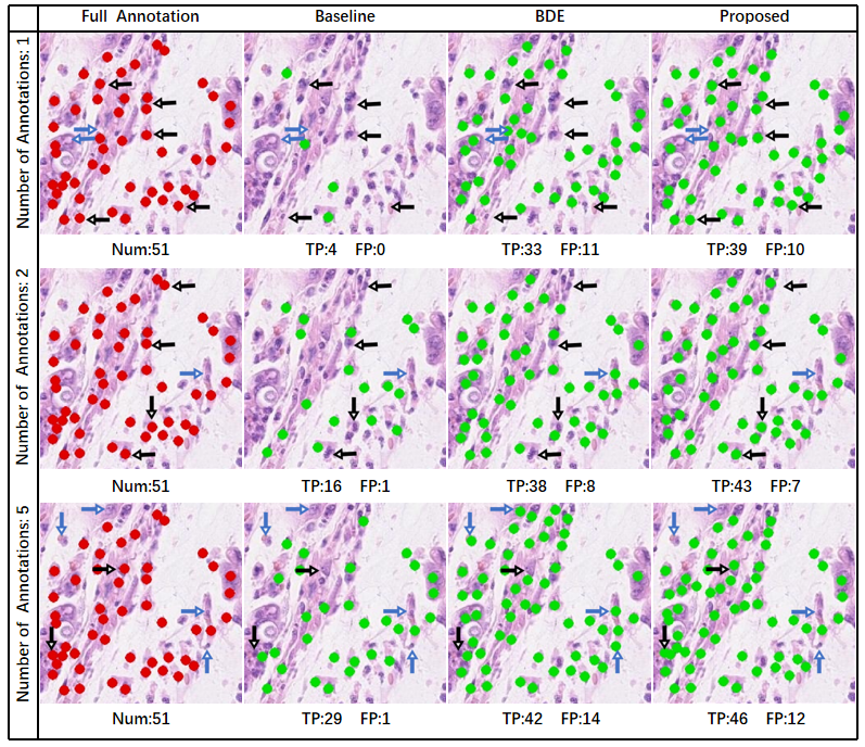
Examples of the detection results of each method on a representative test patch are shown in Fig. 2 for the different cases of annotated cells for training. The complete annotations on the test patch are also shown for reference. Note that since there are a large number of instances in the patch, for the visualization purpose, only the centers of the bounding boxes are shown in Fig. 2 as dots. The numbers of true positive and false positive detection results on the patch are indicated for each method and each case. The baseline method only detected a very small fraction of the cells of interest, which are much fewer than the results of BDE and the proposed method. Compared with the BDE results, the detection results given by the proposed method better match the gold standard full annotations, and the proposed method produced more true positives and fewer false positives for the examples.
Quantitatively, for each fold we computed the average recall, average precision, and average F1-score of the detection results on the test set, and we also computed the corresponding upper bound performance. These results are shown in Tables 7 and 8 for each method and each case of annotated cells. In all cases, the proposed method has higher recall, precision, and F1-score than the two competing approaches, and the results of our method are closer to the upper bound. The means and standard deviations of the average recall, average precision, and average F1-score of the five folds were also computed and are summarized in Table 9, where the proposed method is compared with the competing methods using paired Student’s -tests. In most cases, the proposed method statistically significantly outperforms the competing methods.
| Number of | Method | Fold 1 | Fold 2 | Fold 3 | Fold 4 | Fold 5 | |||||
| Annotations | Recall | Precision | Recall | Precision | Recall | Precision | Recall | Precision | Recall | Precision | |
| 1 | Baseline | 0.112 | 0.101 | 0.115 | 0.098 | 0.103 | 0.096 | 0.098 | 0.091 | 0.112 | 0.091 |
| BDE | 0.524 | 0.462 | 0.501 | 0.421 | 0.574 | 0.471 | 0.620 | 0.554 | 0.521 | 0.464 | |
| Proposed | 0.545 | 0.470 | 0.530 | 0.463 | 0.599 | 0.471 | 0.625 | 0.559 | 0.537 | 0.473 | |
| 2 | Baseline | 0.120 | 0.105 | 0.131 | 0.101 | 0.092 | 0.101 | 0.147 | 0.091 | 0.146 | 0.098 |
| BDE | 0.534 | 0.475 | 0.527 | 0.462 | 0.574 | 0.473 | 0.606 | 0.551 | 0.536 | 0.474 | |
| Proposed | 0.557 | 0.484 | 0.554 | 0.478 | 0.605 | 0.539 | 0.628 | 0.557 | 0.551 | 0.487 | |
| 5 | Baseline | 0.204 | 0.198 | 0.213 | 0.241 | 0.265 | 0.256 | 0.274 | 0.260 | 0.208 | 0.253 |
| BDE | 0.556 | 0.483 | 0.577 | 0.471 | 0.631 | 0.522 | 0.654 | 0.560 | 0.581 | 0.485 | |
| Proposed | 0.562 | 0.488 | 0.598 | 0.486 | 0.638 | 0.532 | 0.667 | 0.566 | 0.592 | 0.489 | |
| - | Upper Bound | 0.671 | 0.601 | 0.682 | 0.612 | 0.696 | 0.629 | 0.701 | 0.639 | 0.689 | 0.605 |
| Number of | Method | F1-score | ||||
| Annotations | Fold 1 | Fold 2 | Fold 3 | Fold 4 | Fold 5 | |
| 1 | Baseline | 0.101 | 0.112 | 0.105 | 0.095 | 0.096 |
| BDE | 0.489 | 0.451 | 0.521 | 0.582 | 0.483 | |
| Proposed | 0.501 | 0.490 | 0.530 | 0.591 | 0.497 | |
| 2 | Baseline | 0.115 | 0.116 | 0.103 | 0.108 | 0.112 |
| BDE | 0.507 | 0.487 | 0.512 | 0.571 | 0.502 | |
| Proposed | 0.513 | 0.508 | 0.564 | 0.596 | 0.519 | |
| 5 | Baseline | 0.205 | 0.221 | 0.257 | 0.269 | 0.228 |
| BDE | 0.517 | 0.519 | 0.581 | 0.606 | 0.523 | |
| Proposed | 0.524 | 0.532 | 0.587 | 0.614 | 0.530 | |
| - | Upper Bound | 0.634 | 0.645 | 0.661 | 0.669 | 0.644 |
| Number of | Method | Recall | Precision | F1-score | ||||||
| Annotations | mean | std | mean | std | mean | std | ||||
| 1 | Baseline | 0.108 | 0.044 | *** | 0.095 | 0.047 | *** | 0.102 | 0.006 | *** |
| BDE | 0.548 | 0.055 | * | 0.474 | 0.052 | n.s. | 0.505 | 0.044 | * | |
| Proposed | 0.567 | 0.060 | - | 0.487 | 0.048 | - | 0.522 | 0.037 | - | |
| 2 | Baseline | 0.127 | 0.020 | *** | 0.099 | 0.004 | *** | 0.111 | 0.005 | *** |
| BDE | 0.556 | 0.030 | ** | 0.487 | 0.032 | n.s. | 0.515 | 0.029 | * | |
| Proposed | 0.579 | 0.031 | - | 0.509 | 0.032 | - | 0.540 | 0.034 | - | |
| 5 | Baseline | 0.233 | 0.030 | *** | 0.242 | 0.023 | *** | 0.236 | 0.024 | *** |
| BDE | 0.600 | 0.037 | * | 0.504 | 0.033 | * | 0.549 | 0.037 | ** | |
| Proposed | 0.611 | 0.037 | - | 0.512 | 0.032 | - | 0.558 | 0.036 | - | |
| - | Upper Bound | 0.688 | 0.011 | - | 0.617 | 0.015 | - | 0.651 | 0.013 | - |
3.4 Results on the TUPAC dataset
We then present the detection results on the TUPAC dataset. As described in Section 3.1.3, the detection model was trained on the training and validation sets with the generated incomplete annotations. The candidate values of the class prior ranged from 0.02 to 0.07 with an increment of 0.01, and was selected based on the validation set.
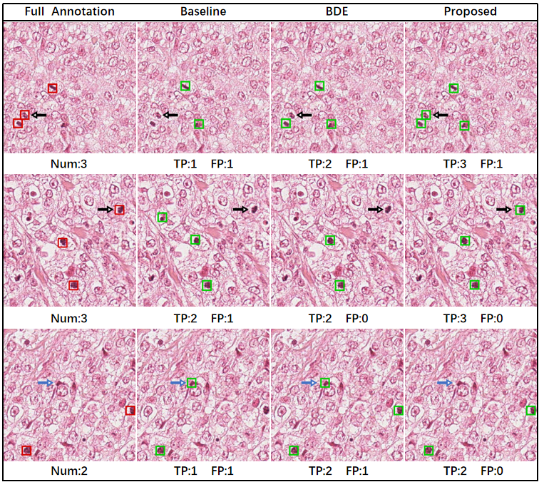
An example of the detection results of the proposed and competing methods is shown in Fig. 3. The bounding boxes predicted by each method are displayed, together with the complete annotations for reference. The numbers of true positive and false positive detection results on the patch are indicated for each method. Our method performs better than the competing methods with fewer false positives or more true positive boxes.
For quantitative evaluation, we computed the means and standard deviations of the recall, precision, and F1-score of the detection results on the test set for each method. Also, the upper bound performance achieved with the complete annotations for training was computed. These results are shown in Table 10. Compared with the competing methods, the proposed method has higher recall, precision, and F1-score, and the results of our method are closer to the upper bound. In addition, in Table 10 the results of the proposed and competing methods are compared using paired Student’s -tests, and the improvement of our method is statistically significant. These observations indicate the better detection performance of the proposed method.
| Method | Recall | Precision | F1-score | ||||||
| mean | std | mean | std | mean | std | ||||
| Baseline | 0.732 | 0.075 | ** | 0.552 | 0.063 | * | 0.623 | 0.067 | * |
| BDE | 0.748 | 0.079 | * | 0.578 | 0.072 | * | 0.652 | 0.068 | * |
| Proposed | 0.760 | 0.082 | - | 0.596 | 0.068 | - | 0.667 | 0.064 | - |
| Upper Bound | 0.775 | 0.056 | - | 0.654 | 0.061 | - | 0.708 | 0.057 | - |
3.5 Results on the NuCLS dataset
Finally, we present the results of multi-class cell detection on the NuCLS dataset. The candidate values of the class prior (for the tumor class) ranged from 0.2 to 0.4 with an increment of 0.05, and was selected based on the validation set.
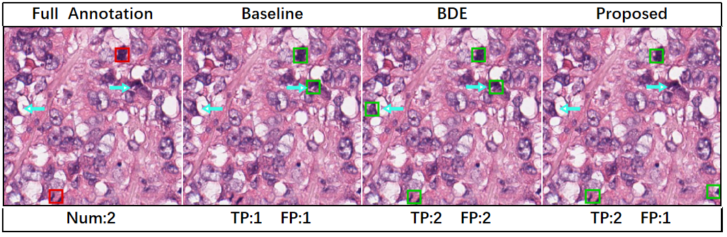
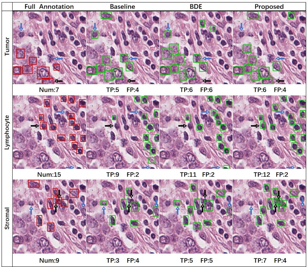
Examples of the detection results of each method on a representative test image are shown in Fig. 4, where the complete annotations are also shown for reference. Because of the large number of instances of each cell type, here the results are shown for each type separately. The numbers of true positive and false positive detection results on the image are indicated for each method. In the given examples, compared with the competing methods, for each cell type our method either produced more true positive boxes without increasing the number of false positives or produced fewer false positive boxes without decreasing the number of true positives.
For quantitative evaluation, we computed the means and standard deviations of the recall, precision, and F1-score of the detection results on the test set for each cell type. The results are shown in Table 11, and the upper bound performance is also given for reference. For all three cell types, the proposed method has higher recall, precision, and F1-score than the two competing approaches. In addition, in Table 11 the proposed method is compared with the competing methods using paired Student’s -tests. In most cases, the recall of the proposed method is significantly better than those of the competing methods; also, for the tumor cells the improvement of the proposed method is significant in most cases.
| Cell Type | Method | Recall | Precision | F1-score | ||||||
| mean | std | mean | std | mean | std | |||||
| Tumor | Baseline | 0.636 | 0.041 | ** | 0.511 | 0.046 | n.s. | 0.566 | 0.044 | * |
| BDE | 0.650 | 0.058 | ** | 0.529 | 0.066 | * | 0.583 | 0.063 | ** | |
| Proposed | 0.689 | 0.043 | - | 0.538 | 0.058 | - | 0.605 | 0.053 | - | |
| Upper Bound | 0.710 | 0.041 | - | 0.622 | 0.040 | - | 0.664 | 0.041 | - | |
| Lymphocyte | Baesline | 0.526 | 0.087 | * | 0.379 | 0.067 | n.s. | 0.440 | 0.064 | n.s. |
| BDE | 0.540 | 0.084 | n.s. | 0.370 | 0.049 | n.s. | 0.438 | 0.055 | n.s. | |
| Proposed | 0.545 | 0.077 | - | 0.389 | 0.046 | - | 0.454 | 0.051 | - | |
| Upper Bound | 0.560 | 0.062 | - | 0.401 | 0.038 | - | 0.467 | 0.045 | - | |
| Stromal | Basleine | 0.388 | 0.046 | * | 0.291 | 0.047 | n.s. | 0.331 | 0.046 | n.s. |
| BDE | 0.409 | 0.041 | ** | 0.280 | 0.025 | n.s. | 0.333 | 0.028 | n.s. | |
| Proposed | 0.436 | 0.045 | - | 0.293 | 0.044 | - | 0.350 | 0.042 | - | |
| Upper Bound | 0.412 | 0.043 | - | 0.319 | 0.031 | - | 0.359 | 0.026 | - | |
4 Discussion
Compared with the BDE method developed in Li et al. (2020) and its extended journal version (Li et al., 2021), our approach addresses the problem of incomplete annotations for cell detection in histopathology images with a principled PU learning framework, and this PU learning framework has led to improved detection performance. Note that our method and the BDE method could be complementary. Based on the density of bounding boxes, it is possible to identify additional negative samples from the unlabeled samples, which may further benefit the training of the detector, and future work could explore the integration of PU learning with the BDE method.
Because in detection problems positively labeled samples and unlabeled samples originate from the same images, in the proposed method the classification loss is approximated differently from the approximation in PU learning for classification problems. The results reported in Section 3.2.2 confirm the benefit of the approximation we have designed for detection problems and support our discussion in Section 2.2.1.
The proposed PU learning strategy was integrated with Faster R-CNN (Ren et al., 2017) for demonstration, because it is a popular CNN-based object detector for cell detection problems (Srinidhi et al., 2021). In addition, we have shown that the proposed method can be applied to different backbones of Faster R-CNN, including the VGG16, ResNet50, and ResNet101 backbones. Since the proposed method is agnostic to the architecture of the detection network, it may also be integrated with more advanced detection networks (Cai and Vasconcelos, 2021; Zhu et al., 2021) that are recently developed, and it would be interesting to investigate in future work whether such integration can lead to improved performance.
In addition to PU learning for binary cell detection, we have extended the proposed framework to multi-class cell detection. Multi-class PU learning has also been investigated before for classification (Xu et al., 2017; Shu et al., 2020), but not for cell detection. The experimental results on the NuCLS dataset show that our method allows improved multi-class cell detection given incomplete annotations.
The problem of incomplete annotations considered in the proposed work is related to but different from semi-supervised learning. For both semi-supervised learning and the proposed work, not all cells of interest are annotated on the training images. However, they are different in terms of how the training data is obtained. In semi-supervised learning every cell of interest should be annotated for the labeled data. For detection problems, this can be more challenging than incomplete annotations, because it requires that experts carefully examine the annotation results to ensure that no cells of interest are left unannotated in the labeled data, whereas for incomplete annotations no such burden is required.
5 Conclusion
We have proposed to apply PU learning to address the problem of network training with incomplete annotations for cell detection in histopathology images. In our method, the classification loss is more appropriately computed from the incompletely annotated data during network training for both binary and multi-class cell detection. The experimental results on four publicly available datasets show that our method can improve the performance of cell detection in histopathology images given incomplete annotations.
Acknowledgments
This work is supported by National Natural Science Foundation of China (62001009).
Ethical Standards
The work follows appropriate ethical standards in conducting research and writing the manuscript, following all applicable laws and regulations regarding treatment of animals or human subjects.
Conflicts of Interest
We declare we don’t have conflicts of interest.
References
- Amgad et al. (2021) Mohamed Amgad, Lamees A. Atteya, Hagar Hussein, Kareem Hosny Mohammed, Ehab Hafiz, Maha A. T. Elsebaie, Ahmed M. Alhusseiny, Mohamed Atef AlMoslemany, Abdelmagid M. Elmatboly, Philip A. Pappalardo, Rokia Adel Sakr, Pooya Mobadersany, Ahmad Rachid, Anas M. Saad, Ahmad M. Alkashash, Inas A. Ruhban, Anas Alrefai, Nada M. Elgazar, Ali Abdulkarim, Abo-Alela Farag, Amira Etman, Ahmed G. Elsaeed, Yahya Alagha, Yomna A. Amer, Ahmed M. Raslan, Menatalla K. Nadim, Mai A. T. Elsebaie, Ahmed Ayad, Liza E. Hanna, Ahmed M. Gadallah, Mohamed Elkady, Bradley Drumheller, David Jaye, David Manthey, David A. Gutman, Habiba Elfandy, and Lee A. D. Cooper. NuCLS: A scalable crowdsourcing, deep learning approach and dataset for nucleus classification, localization and segmentation. arXiv preprint arXiv:2102.09099, 2021.
- Bertram et al. (2020) Christof A. Bertram, Mitko Veta, Christian Marzahl, Nikolas Stathonikos, Andreas Maier, Robert Klopfleisch, and Marc Aubreville. Are pathologist-defined labels reproducible? comparison of the TUPAC16 mitotic figure dataset with an alternative set of labels. In Interpretable and Annotation-Efficient Learning for Medical Image Computing, pages 204–213, 2020.
- Cai et al. (2019) De Cai, Xianhe Sun, Niyun Zhou, Xiao Han, and Jianhua Yao. Efficient mitosis detection in breast cancer histology images by RCNN. In International Symposium on Biomedical Imaging, pages 919–922, 2019.
- Cai and Vasconcelos (2021) Zhaowei Cai and Nuno Vasconcelos. Cascade R-CNN: High quality object detection and instance segmentation. IEEE Transactions on Pattern Analysis and Machine Intelligence, 43(5):1483–1498, 2021.
- Deng et al. (2009) Jia Deng, Wei Dong, Richard Socher, Li-Jia Li, Kai Li, and Li Fei-Fei. ImageNet: A large-scale hierarchical image database. In IEEE Conference on Computer Vision and Pattern Recognition, pages 248–255, 2009.
- Elkan and Noto (2008) Charles Elkan and Keith Noto. Learning classifiers from only positive and unlabeled data. In International Conference on Knowledge Discovery and Data Mining, pages 213–220, 2008.
- Fusi et al. (2013) Alberto Fusi, Robert Metcalf, Matthew Krebs, Caroline Dive, and Fiona Blackhall. Clinical utility of circulating tumour cell detection in non-small-cell lung cancer. Current Treatment Options in Oncology, 14(4):610–622, 2013.
- Gurcan et al. (2009) Metin N Gurcan, Laura E Boucheron, Ali Can, Anant Madabhushi, Nasir M Rajpoot, and Bulent Yener. Histopathological image analysis: A review. IEEE Reviews in Biomedical Engineering, 2:147–171, 2009.
- He et al. (2016) Kaiming He, Xiangyu Zhang, Shaoqing Ren, and Jian Sun. Deep residual learning for image recognition. In IEEE Conference on Computer Vision and Pattern Recognition, pages 770–778, 2016.
- He et al. (2021) Yunjie He, Hong Zhao, and Stephen T. C. Wong. Deep learning powers cancer diagnosis in digital pathology. Computerized Medical Imaging and Graphics, 88:101820, 2021.
- Kingma and Ba (2014) Diederik P Kingma and Jimmy Ba. Adam: A method for stochastic optimization. arXiv preprint arXiv:1412.6980, 2014.
- Kiryo et al. (2017) Ryuichi Kiryo, Gang Niu, Marthinus C. du Plessis, and Masashi Sugiyama. Positive-unlabeled learning with non-negative risk estimator. In Advances in Neural Information Processing Systems, pages 1674–1684, 2017.
- Li et al. (2020) Hansheng Li, Xin Han, Yuxin Kang, Xiaoshuang Shi, Mengdi Yan, Zixu Tong, Qirong Bu, Lei Cui, Jun Feng, and Lin Yang. A novel loss calibration strategy for object detection networks training on sparsely annotated pathological datasets. In International Conference on Medical Image Computing and Computer-Assisted Intervention, pages 320–329, 2020.
- Li et al. (2021) Hansheng Li, Yuxin Kang, Wentao Yang, Zhuoyue Wu, Xiaoshuang Shi, Liu Feihong, Jianye Liu, Lingyu Hu, Qian Ma, Lei Cui, Jun Feng, and Lin Yang. A robust training method for pathological cellular detector via spatial loss calibration. Frontiers in Medicine, 8:767625, 2021.
- Li et al. (2019) Jiahui Li, Shuang Yang, Xiaodi Huang, Qian Da, Xiaoqun Yang, Zhiqiang Hu, Qi Duan, Chaofu Wang, and Hongsheng Li. Signet ring cell detection with a semi-supervised learning framework. In International Conference on Information Processing in Medical Imaging, pages 842–854, 2019.
- Lin et al. (2017) Tsung-Yi Lin, Priya Goyal, Ross Girshick, Kaiming He, and Piotr Dollár. Focal loss for dense object detection. In International Conference on Computer Vision, pages 2980–2988, 2017.
- Lu et al. (2021) Ming Y Lu, Tiffany Y Chen, Drew F K Williamson, Melissa Zhao, Maha Shady, Jana Lipkova, and Faisal Mahmood. AI-based pathology predicts origins for cancers of unknown primary. Nature, 594(7861):106–110, 2021.
- Marostica et al. (2021) Eliana Marostica, Rebecca Barber, Thomas Denize, Isaac S Kohane, Sabina Signoretti, Golden A Jeffrey, and Kun-Hsing Yu. Development of a histopathology informatics pipeline for classification and prediction of clinical outcomes in subtypes of renal cell carcinoma. Clinical Cancer Research, 27(10):2868–2878, 2021.
- Neubeck and Van Gool (2006) Alexander Neubeck and Luc Van Gool. Efficient non-maximum suppression. In International Conference on Pattern Recognition, pages 850–855, 2006.
- Noorbakhsh et al. (2020) Javad Noorbakhsh, Saman Farahmand, Ali Foroughi Pour, Sandeep Namburi, Dennis Caruana, David Rimm, Mohammad Soltanieh-ha, Kourosh Zarringhalam, and Jeffrey H Chuang. Deep learning-based cross-classifications reveal conserved spatial behaviors within tumor histological images. Nature Communications, 11:6367, 2020.
- Ren et al. (2017) Shaoqing Ren, Kaiming He, Ross Girshick, and Jian Sun. Faster R-CNN: Towards real-time object detection with region proposal networks. IEEE Transactions on Pattern Analysis and Machine Intelligence, 39(6):1137–1149, 2017.
- Roux et al. (2013) Ludovic Roux, Daniel Racoceanu, Nicolas Loménie, Kulikova Maria, Humayun Irshad, Jacques Klossa, Frédérique Capron, Catherine Genestie, Le Gilles Naour, and Metin N Gurcan. Mitosis detection in breast cancer histological images An ICPR 2012 contest. Journal of Pathology Informatics, 4:8, 2013.
- Shu et al. (2020) Senlin Shu, Zhuoyi Lin, Yan Yan, and Li Li. Learning from multi-class positive and unlabeled data. In International Conference on Data Mining, pages 1256–1261, 2020.
- Simonyan and Zisserman (2015) Karen Simonyan and Andrew Zisserman. Very deep convolutional networks for large-scale image recognition. arXiv preprint arXiv:1409.1556, 2015.
- Sirinukunwattana et al. (2016) Korsuk Sirinukunwattana, Shan E Ahmed Raza, Yee-Wah Tsang, David R. J. Snead, Ian A. Cree, and Nasir M. Rajpoot. Locality sensitive deep learning for detection and classification of nuclei in routine colon cancer histology images. IEEE Transactions on Medical Imaging, 35(5):1196–1206, 2016.
- Srinidhi et al. (2021) Chetan L. Srinidhi, Ozan Ciga, and Anne L. Martel. Deep neural network models for computational histopathology: A survey. Medical Image Analysis, 67:101813, 2021.
- Sun et al. (2020) Yibao Sun, Xingru Huang, Edgar Giussepi Lopez Molina, Le Dong, and Qianni Zhang. Signet ring cells detection in histology images with similarity learning. In International Symposium on Biomedical Imaging, pages 490–494, 2020.
- Tomczak et al. (2015) Katarzyna Tomczak, Patrycja Czerwinska, and Maciej Wiznerowicz. The cancer genome atlas (TCGA): An immeasurable source of knowledge. Contemporary Oncology, 19(1A):A68–A77, 2015.
- van der Laak et al. (2021) Jeroen van der Laak, Geert Litjens, and Francesco Ciompi. Deep learning in histopathology: the path to the clinic. Nature Medicine, 27:775–784, 2021.
- Veta et al. (2014) Mitko Veta, Josien P. W. Pluim, Paul J. van Diest, and Max A. Viergever. Breast cancer histopathology image analysis: A review. IEEE Transactions on Biomedical Engineering, 61(5):1400–1411, 2014.
- Veta et al. (2019) Mitko Veta, J. Heng Yujing, Nikolas Stathonikos, Babak Bejnordi Ehteshami, Francisco Beca, Thomas Wollmann, Karl Rohr, A. Shah Manan, Dayong Wang, Mikael Rousson, Martin Hedlund, David Tellez, Francesco Ciompi, Erwan Zerhouni, David Lanyi, Matheus Viana, Vassili Kovalev, Vitali Liauchuk, Hady Ahmady Phoulady, Talha Qaiser, Simon Graham, Nasir Rajpoot, Erik Sjöblom, Jesper Molin, Kyunghyun Paeng, Sangheum Hwang, Sunggyun Park, Zhipeng Jia, Eric I-Chao Chang, Yan Xu, Andrew H. Beck, Paul J. van Diest, and Josien P.W. Pluim. Predicting breast tumor proliferation from whole-slide images: The TUPAC16 challenge. Medical Image Analysis, 54:111–121, 2019.
- Wang et al. (2022) Ching-Wei Wang, Sheng-Chuan Huang, Yu-Ching Lee, Yu-Jie Shen, Shwu-Ing Meng, and Jeff L. Gaol. Deep learning for bone marrow cell detection and classification on whole-slide images. Medical Image Analysis, 75:102270, 2022.
- Xu et al. (2016) Jun Xu, Lei Xiang, Qingshan Liu, Hannah Gilmore, Jianzhong Wu, Jinghai Tang, and Anant Madabhushi. Stacked sparse autoencoder (SSAE) for nuclei detection on breast cancer histopathology images. IEEE Transactions on Medical Imaging, 35(1):119–130, 2016.
- Xu et al. (2017) Yixing Xu, Chang Xu, Chao Xu, and Dacheng Tao. Multi-positive and unlabeled learning. In International Joint Conference on Artificial Intelligence, pages 3182–3188, 2017.
- Yang et al. (2020) Yuewei Yang, Kevin J Liang, and Lawrence Carin. Object detection as a positive-unlabeled problem. In British Machine Vision Conference, 2020.
- Zhao et al. (2021) Zipei Zhao, Fengqian Pang, Zhiwen Liu, and Chuyang Ye. Positive-unlabeled learning for cell detection in histopathology images with incomplete annotations. In International Conference on Medical Image Computing and Computer-Assisted Intervention, pages 509–518, 2021.
- Zhu et al. (2021) Xizhou Zhu, Weijie Su, Lewei Lu, Bin Li, Xiaogang Wang, and Jifeng Dai. Deformable DETR: Deformable transformers for end-to-end object detection. In International Conference on Learning Representations, 2021.
Appendix A A Baseline performance achieved with the weighted cross entropy loss or focal loss
In this appendix, we present the results of the baseline method achieved with the weighted cross entropy loss and the focal loss (Lin et al., 2017) for the experiment on the MITOS-ATYPIA-14 dataset with the experimental settings specified for Section 3.2.1. The weighted cross entropy loss and the focal loss are defined as
| (16) | |||||
| (17) |
Here, is a weight for the positive class in the weighted cross entropy loss that alleviates the problem of class imbalance, and we set ; and are the parameters for the focal loss that balance the importance of positive/negative samples and easy/hard samples, respectively, and we set and according to Lin et al. (2017).
The detection performance achieved with the weighted cross entropy loss and focal loss is summarized in Table A1, where the means and standard deviations of the average recall, average precision, and average F1-score of the five folds are listed. Compared with the baseline results achieved with the standard cross entropy loss in Table 3, the use of the two alternative losses did not lead to improved detection performance (the F1-score is reduced).
| Loss | Recall | Precision | F1-score |
| Weighted Cross Entropy | 0.6030.079 | 0.3560.026 | 0.4450.034 |
| Focal | 0.5620.091 | 0.3940.032 | 0.4610.048 |
Appendix B B Sensitivity to the class prior
The evaluation of the sensitivity of the detection performance to the class prior is provided in this appendix. We computed the F1-score corresponding to each candidate on the test set for the MITOS-ATYPIA-14 dataset with the experimental settings specified for Section 3.2.1, and the results are shown in Table B1 for each fold. The difference between the best and second best results achieved with different values is small, and both of them are better than the BDE results in Table 2.
| F1-score | |||||
| Fold 1 | Fold 2 | Fold 3 | Fold 4 | Fold 5 | |
| 0.508 | 0.465 | 0.460 | 0.431 | 0.549 | |
| 0.517 | 0.480 | 0.471 | 0.447 | 0.560 | |
| 0.523 | 0.487 | 0.470 | 0.456 | 0.572 | |
| 0.524 | 0.485 | 0.488 | 0.457 | 0.587 | |
| 0.514 | 0.475 | 0.484 | 0.443 | 0.583 | |
| 0.507 | 0.468 | 0.473 | 0.445 | 0.580 | |
Appendix C C The impact of random effects
| Method | Recall | Precision | F1-score |
| Baseline | 0.6050.006 | 0.4120.005 | 0.4910.002 |
| BDE | 0.6390.003 | 0.4310.006 | 0.5150.004 |
| Proposed | 0.6420.006 | 0.4410.006 | 0.5250.005 |
During network training, random effects such as batch selection can lead to different learned network weights. Therefore, we investigated the impact of random effects on the detection performance for the proposed and competing methods using the MITOS-ATYPIA-14 dataset with the experimental settings specified for Section 3.2.1. The baseline method, BDE method, and proposed method were repeated independently five times with the first fold (including the results presented in Section 3.2.1). The means and standard deviations of the recall, precision, and F1-score results of the five runs are shown in Table C1. The standard deviations are relatively small compared with the means, indicating that all methods are robust to random effects, and our method is better than the competing methods with higher recall, precision, and F1-score.