

1 Introduction
Ultrasound b-mode imaging is a qualitative approach and is highly dependent on the operators’ experience. In b-mode imaging, different tissue types can result in very similar image impressions, for example, in breast cancer screening b-mode images have low specificity for differentiating malignant and benign lesions (Carra et al., 2014; Chung and Cho, 2015). This complicates the diagnosis. Quantitative information, e.g., elasticity, density, speed-of-sound (SoS), and attenuation can increase ultrasound specificity and ease interpretation. Studies show that SoS values carry diagnostic information that can be used for tissue characterization (Hachiya et al., 1994; Khodr et al., 2015; Sak et al., 2017; Sanabria et al., 2018a).
Application-specific systems, e.g., ultrasound tomography systems (USCT) have emerged to measure SoS and attenuation in tissues (Duric et al., 2007). There are several methods of reconstruction for USCT, e.g., approximate models such as ray-tracing methods (Jirik et al., 2012; Opieliński et al., 2018; Javaherian et al., 2020; Li et al., 2009, 2010) that are often fast but have low spatial resolutions; or the full-wave inversion (FWI) methods that directly solve the wave equation and allow the whole measured data to be used in the inversion (time-series or all frequencies), thus, resulting in high-resolution images (Wiskin et al., 2007; Roy et al., 2010; Agudo et al., 2018; Li et al., 2014; Wang et al., 2015; Pérez-Liva et al., 2017; Lucka et al., 2021). The drawback of FWI methods is that they have a huge memory footprint and are computationally expensive (Lucka et al., 2021). Additionally, from the hardware point of view, USCT typically needs double-sided access to the tissue with multiple transducers (Malik et al., 2018; Duric et al., 2007; Gemmeke and Ruiter, 2007) which makes the setups bulky and costly.
SoS values can be estimated using conventional pulse-echo setups (Qu et al., 2012; Benjamin et al., 2018; Sanabria et al., 2018a). In practice, SoS in tissue can be estimated in various ways. One method is based on the idea that the assumed SoS used in b-mode image reconstruction closely matches the actual SoS if the b-mode image quality is maximized (Gyöngy and Kollár, 2015; Benjamin et al., 2018). Stähli et al. (2020b) proposed computed ultrasound tomography in echo mode (CUTE). This method is based on spatial phase shifts of beamformed echoes. In Huang and Li (2004); Sanabria et al. (2018b) a passive reflector is used and a limited angle ill-posed inverse problem is formulated. Stähli et al. (2020a) proposed a Bayesian framework to solve the inverse problem which includes an a priori model based on b-mode image segmentation.
Model-based SoS reconstruction is a non-trivial task and extracting SoS information by analytical or optimization methods requires prior knowledge, carefully chosen regularization, and optimization methods (Vishnevskiy et al., 2019). Furthermore, there are challenges in implementing these methods for real-time imaging, only a few methods have the potential to be used in real-time imaging systems (e.g., CUTE (Stähli et al., 2020b)) but often these methods are computationally expensive with varying run times.
Deep-learning-based methods move the computational burden to the training phase and therefore have a great potential for real-time applications. In recent years, these techniques are vastly being used in the medical imaging field (Suzuki, 2017; Lee et al., 2017; Mainak et al., 2019; Maier et al., 2019; Lundervold and Lundervold, 2019; Wang et al., 2018). As such, in the field of medical ultrasound, deep learning techniques are gaining rapid attention, especially for segmentation and image formation (a.k.a. beamforming), an overview can be found in van Sloun et al. (2019); Mischi et al. (2020).
Studies on deep-learning-based quantitative ultrasound are sparse compared to image formation approaches (Vishnevskiy et al., 2019; Hoerig et al., 2018; Feigin et al., 2019, 2020; Khun Jush et al., 2020, 2021; Bernhardt et al., 2020; Gao et al., 2019; Mohammadi et al., 2021; Heller and Schmitz, 2021; Oh et al., 2021). Deep-learning-based SoS reconstruction for pulse-echo ultrasound was first addressed in Feigin et al. (2019). Inspired by Feigin et al. (2019), in Khun Jush et al. (2020) we investigated the possibility of deep-learning-based SoS reconstruction for automated breast ultrasound using a single PW acquisition. These studies rely on simulated training data.
2 Thesis and Aim
One of the main obstacles to developing deep learning techniques is the collection of training datasets alongside their corresponding labels or Ground Truth (GT) maps. This process is often time-consuming and costly. The problem further expands when the labeled data or GT is difficult to measure. Particularly, for SoS reconstruction there is no gold-standard reference method capable of creating SoS GT from ultrasound reflection data. Plus, there are only a few phantoms available with known heterogeneous SoS. Therefore, using simulated data for the training phase is a common approach in deep-learning-based algorithms (Feigin et al., 2019, 2020; Khun Jush et al., 2020, 2021; Vishnevskiy et al., 2019; Oh et al., 2021; Heller and Schmitz, 2021). These studies employed a simplified setup for tissue modeling in which inclusions are assumed to be simple geometric structures, e.g., ellipsoids, randomly located in a homogeneous background.
Although the previously proposed tissue models enabled deep-learning-based SoS reconstruction, the simplified approach does not reflect the complexity of real tissues, thus, resulting in stability and reproducibility challenges when tested on measured data, especially in the presence of noise. We encountered such challenges in Khun Jush et al. (2020) that motivated the current study. Creating large diverse training data is a crucial task. Deep-learning-based models only deal with generalization within the distributions of the training data. Otherwise, the model performs poorly or fails in real-world setups. Therefore, the broader the distribution of the training data the more the likelihood of success of the deep neural networks in real setups. One possibility which is extensively studied is to train the models with pools of different datasets or multiple datasets each providing a different aspect of the underlying model (Goyal and Bengio, 2020).
This study aims to investigate the stability and pitfalls of an existing deep-learning-based method for SoS reconstruction and improve its performance by introducing diversity to tissue modeling. Additionally, since tissue modeling is a non-trivial task, investigations of the sensitivity of the networks are helpful to create a stable setup for data generation which is missing from previous studies. Therefore, we include experiments with digital phantoms of various properties and provide the reader with insights regarding the sensitivity of the investigated network encountering out-of-domain simulation characteristics, e.g., varying echogenicity, geometry, speckle density, and noise.
The contributions of this study are as follows:
- (i)
We proposed a new simulation setup based on Tomosynthesis images to expand the diversity of the tissue modeling that integrates tissue-like structures for ultrasound training data generation.
- (ii)
We augmented the dataset created from our proposed setup to a baseline simplified tissue model proposed by Feigin et al. (2019, 2020) and showed that without any modifications the existing architecture (an encoder-decoder network using a single plane-wave acquisition) is capable of reconstructing the complicated SoS maps as well as simple structures.
- (iii)
We analyzed the stability of the network trained with augmented data in comparison with the baseline setup (simplified tissue model) in the presence of out-of-domain simulated data to find the crucial parameters to which the network shows high sensitivity.
- (iv)
We compared the stability and robustness of the network trained with the simplified dataset versus the augmented dataset on measured phantom data and showed that the network trained with a joint set of data is more stable when tested on real data.
3 Materials and Methods
We used the k-Wave toolbox (Version 1.3) (Treeby and Cox, 2010) for simulating the training data. K-Wave is a MATLAB toolbox that allows simulation of linear and non-linear wave propagation, arbitrary heterogeneous parameters for mediums, and acoustic absorption (Treeby and Cox, 2010). Studies demonstrated that acoustic non-linearity and absorption are well modeled in k-wave, and when there is a good representation of medium properties and geometry, the models are accurate (Wang et al., 2012; Treeby et al., 2012; Martin et al., 2019; Agrawal et al., 2021).
We generated a training dataset using two simulation setups, one based on prior works proposed by Feigin et al. (2019) and one is a new simulation setup that we introduce in this study. We used a single PW and 2D medium of size (grid size: ) where the transducer is placed in the central section of the mediums (for more details on transducer setup, the geometry of the medium and acoustic properties see Appendix A.1 and A.2).
3.1 Simulation Setup
3.1.1 Prior Work: Ellipsoids Setup
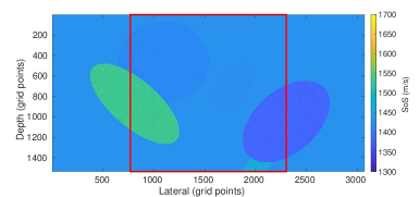
The first setup is a setup based on Feigin et al. (2019) adapted to our transducer properties with 192 active channels and single PW acquisition. The setup is a simplified model for organs and lesions. In this setup, the medium consists of a homogeneous background with elliptical inclusions randomly located in the medium where the SoS values are assigned randomly in the range . Although the expected SoS in the breast tissue is in a smaller range (Li et al., 2009), the higher range (i.e., ) is chosen for better generalization (Feigin et al., 2019). Details of the simulation parameters for this setup are added in Appendix A.3. This setup is considered as a baseline setup for comparison purposes. Henceforth, we refer to this setup as Ellipsoids setup, an example of this setup is shown in Figure 1.
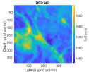
3.1.2 Proposed Setup: Tomosynthesis to Ultrasound (T2US)
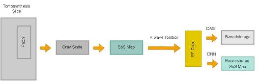
Here we introduce a new simulation setup that includes more complicated structures in the mediums. The intensity of CT images that are measured in the Hounsfield units (HU) is related to tissue density. SoS and attenuation of the tissues are directly related to the density as well. Therefore, the idea of simulating ultrasound images from CT images was investigated in prior studies (Dillenseger et al., 2009; Shams et al., 2008; Cong et al., 2013; Kutter et al., 2009; Sak et al., 2017) but in the context of developing fast ultrasound simulations due to the high computational demands of standard acoustic simulation setups. However, since the k-wave toolbox supports GPU and CPU acceleration, it has a decent run time on modern Nvidia GPUs. Plus, we use a single PW and 2D grid. Therefore, we propose a different approach to create ultrasound images from CT images. The proposed method extracts the underlying tissue-like structures from Tomosynthesis images and creates heterogeneous SoS mediums for the standard k-wave simulation.
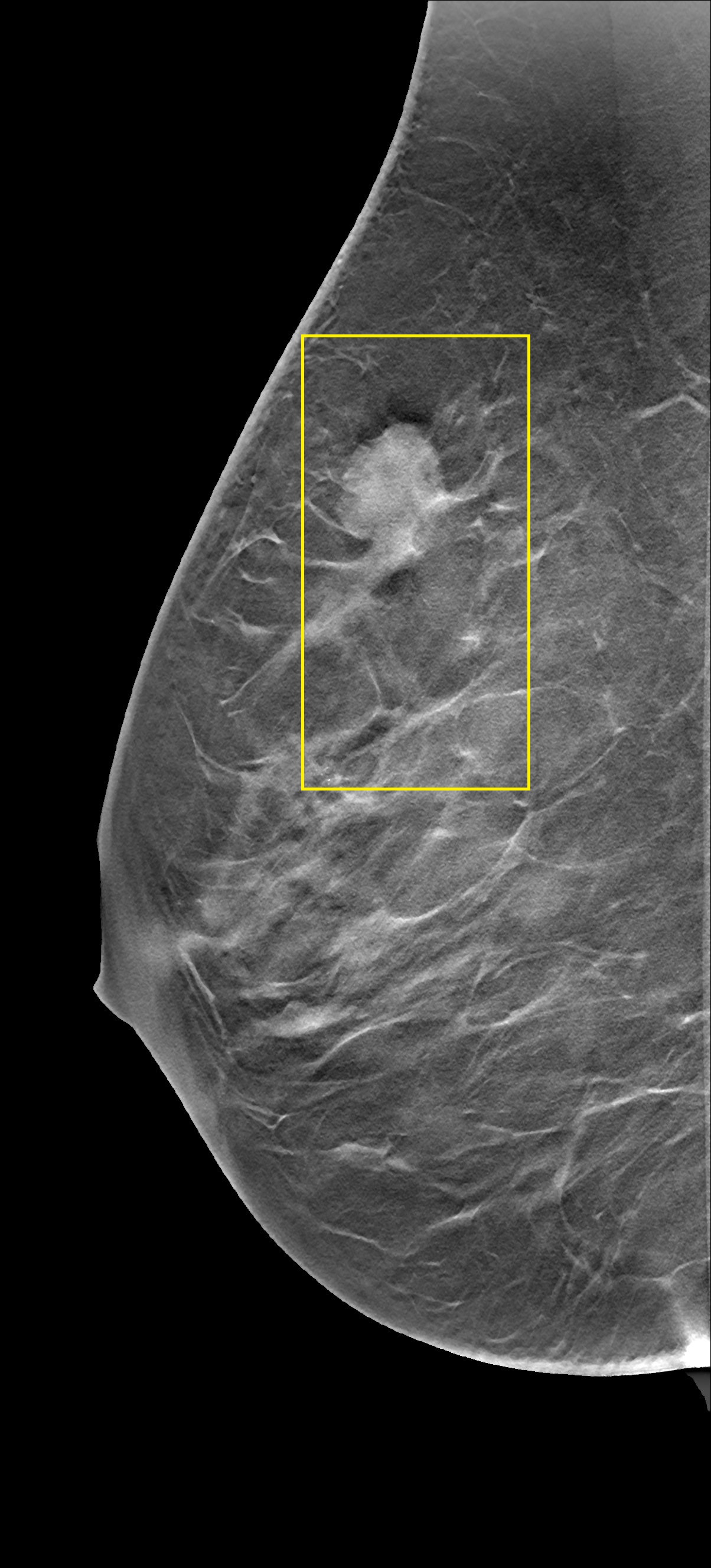
14 Tomosynthesis image stacks are used. Each image stack contains between 29 to 74 slices. These images are acquired from patients diagnosed with benign or malignant breast lesions.
 | |
| (a) | |
 (b) (b) | 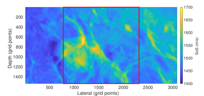 (c) (c)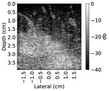 (d) (d) |
SoS Map
From each slice, 10 patches with size pixels are randomly extracted. Patches are chosen in a way that the black regions outside the breast area present in the Tomosynthesis slices are excluded. Overlapping regions in the patches from the same slide are not excluded. In order to reduce the range, HU values are converted to grayscale values. Because of the presence of modality noise in Tomosynthesis images, the patches are smoothed with a 2D Gaussian smoothing kernel with a standard deviation of . The patches are resized to fit the medium size using nearest-neighbor interpolation.
The grayscale values are then mapped to SoS in the range (rescale function of MATLAB from Data Import and Analysis, Preprocessing Data toolbox is used). Currently, in order to define malignancy, solid breast lesions are examined based on the qualitative analysis of tumor margins and geometry (e.g., speculation, boundary uniformity, ovality). Studies suggest that the echogenicity of the lesion on its own does not provide enough contrast for differentiation (Blickstein et al., 1995; Ruby et al., 2019). Nevertheless, there is an echogenicity contrast present between lesions and fatty tissues (Gokhale, 2009). Thus, we included random hyperechogenic regions. Based on the mapped SoS, echogenicity of of the pixels with assigned values higher than , or lower than varies by for half of the cases. This intends to create varying echogenicity independent of the presence of a lesion. These patches are given to the simulation as the SoS domain.
It is noteworthy that the assigned SoS values are not intended to reflect real corresponding SoS values to a particular tissue type present in the Tomosynthesis image, but the aim is to include more detailed structures rather than geometric shapes used in the Ellipsoids setup. An overview is shown in Figure 2.
3.2 Deep Neural Network
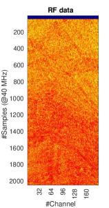
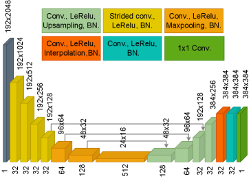
The network architecture is based on Feigin et al. (2019, 2020) adopted to a transducer geometry with 192 active channels presented in Khun Jush et al. (2020). The network is a fully convolutional neural network (FCNN), encoder-decoder network. The input of the network is RF data from a single PW acquisition, sampled at (in form of a matrix of , bit floating point). The output of the network is the predicted SoS map presented as a matrix with resolution. The network architecture is shown in Figure 3. The contracting and extracting paths each contain seven layers. The details of the operations in each layer are color-coded in Figure 3 (b).
3.3 Experimental Setup
The network is trained only on simulated data and tested both on simulated and measured data acquired from a commercial breast phantom, CIRS multi-modality breast biopsy, and sonographic trainer (Model 073). This phantom mimics breast tissue properties with heterogeneous SoS, density, and attenuation. The data is acquired with the LightABVS prototype system presented in Hager et al. (2019); Khun Jush et al. (2020).
4 Results and Discussion
In this section, first of all, we will show the results of the networks trained with simulated datasets and compare the performance of the encoder-decoder network on different training data pools. Afterward, we investigate the stability of the trained networks in the presence of out-of-domain simulated data and noise to pinpoint the sensitivity of the network to different acoustic parameters. Moreover, experimental results from the CIRS phantom are included and the reproducibility and stability of the networks are discussed.
4.1 Simulated Data
4.1.1 Training Data


Selecting the size of the training dataset for a network is a non-trivial task. In order to select the required size, we have trained the network on training sets of 2000, 3000, 4000, 5000, and 6000 cases of the Ellipsoids dataset and observed that there is a saturation of the performance and increasing the number of training cases does not improve the performance even on the simulated dataset. Figure 4 demonstrates this fact by comparing the learning curves for training and validation sets of varying sizes. This implies that increasing the number of training samples of the same kind of simulated data is not the optimal solution to improve the performance of the network. There are two options to improve the performance of the network, one is to modify the network architecture and the other is to improve the quality and diversity of the training set. Here, we focus on the second approach.
The network is trained with three sets of input datasets: Ellipsoids setup and T2US setup to show that the network is capable of reconstructing each dataset, and combined sets of two aforementioned datasets to show that the network can learn two mappings jointly. The stability study focuses on the combined dataset compared to the baseline simplified model.
For each simulation setup, samples are simulated. The dataset is divided to train ( for training and for validation) and test cases. For more information regarding training and data processing see Appendix B. The network is trained for 150 epochs for Ellipsoids and T2US setups and 200 epochs for the Combined setup using mini-batch stochastic gradient descent and MSE loss function. Table 1 shows the corresponding error rates on the test datasets after convergence.
Sample cases of qualitative results for Ellipsoids, T2US, and Combined setups are shown in Figure 5. In order to compare qualitative cases, their corresponding RMSE, MAE, and structural similarity index (a.k.a. SSIM (Wang et al., 2004)) values are added below each case in Figure 5.
| Dataset | RMSE SD (m/s) | MAE SD (m/s) | MAPE SD (%) |
| Ellipsoids | |||
| T2US | |||
| Combined |
| Case 1 | Case 2 | Case 3 | Case 4 | Case 5 | Case 6 | Case 7 | Case 8 | Case 9 | Case 10 | [m/s] | |
| GT |  |  |  | 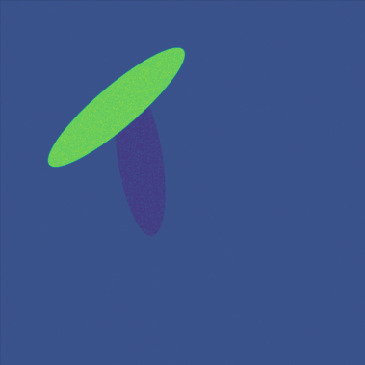 |  | 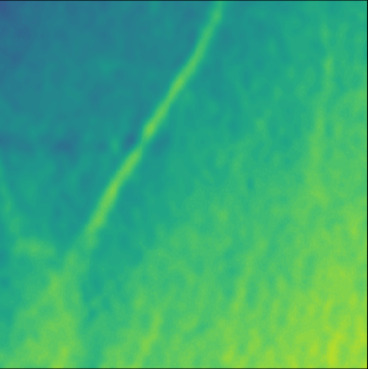 | 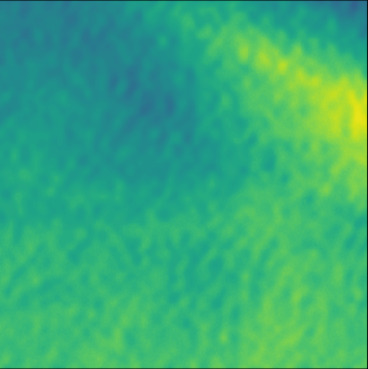 | 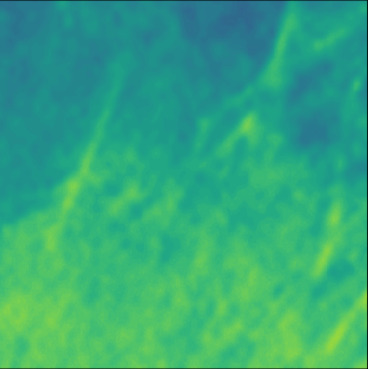 | 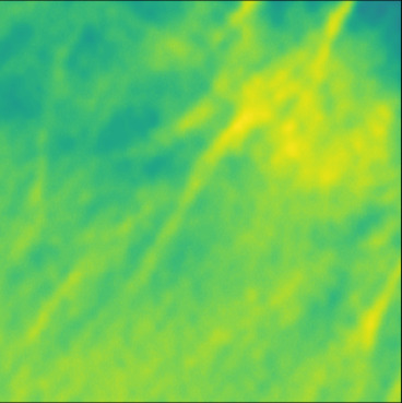 | 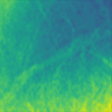 | |
| PredictedSoS | 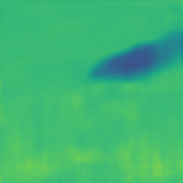 | 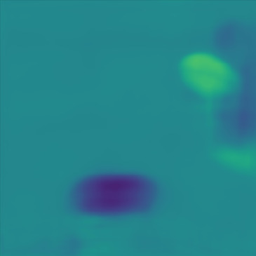 | 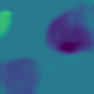 | 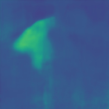 | 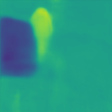 | | 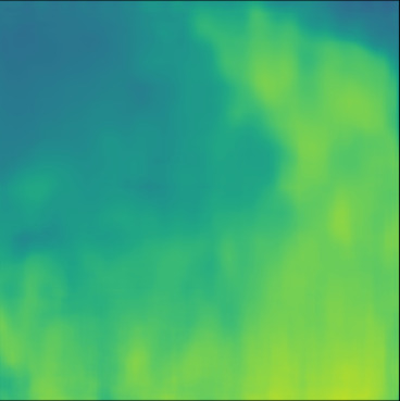 | 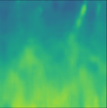 | 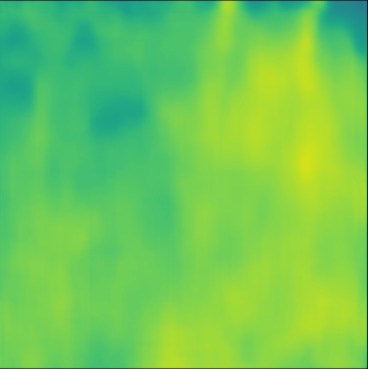 | 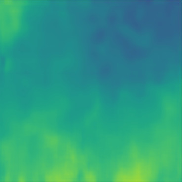 | |
| AbsoluteDifference |  |  |  |  |  |  |  |  | 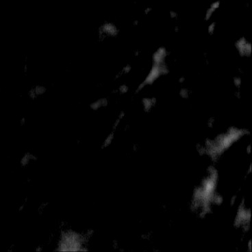 | 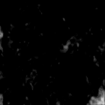 | |
| RMSE | 5.50 | 13.45 | 11.26 | 9.83 | 15.48 | 21.46 | 29.29 | 23.93 | 31.73 | 21.36 | [m/s] |
| MAE | 2.17 | 5.43 | 6.44 | 4.00 | 6.89 | 16.12 | 22.20 | 18.83 | 25.33 | 16.68 | [m/s] |
| SSIM | 0.89 | 0.82 | 0.72 | 0.85 | 0.80 | 0.73 | 0.71 | 0.64 | 0.65 | 0.72 | |
| PredictedSoS | | | | | | 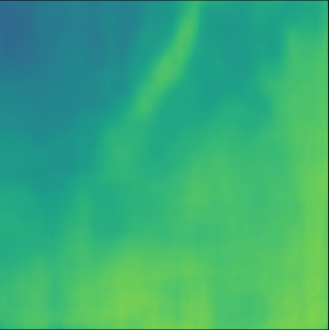 | 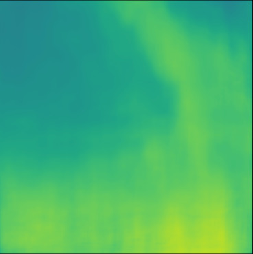 | 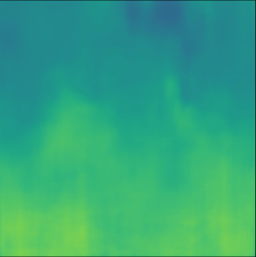 | 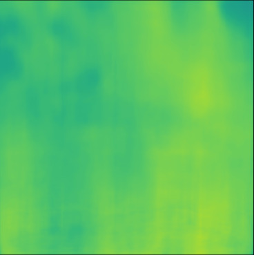 | 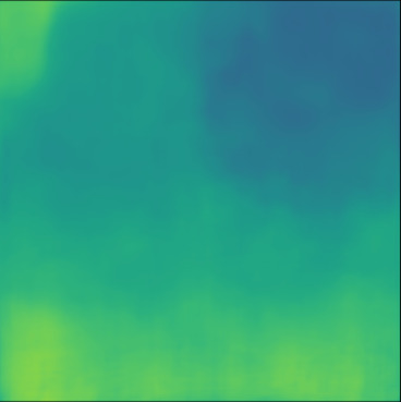 | |
| AbsoluteDifference | | | | | |  | 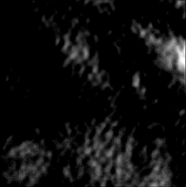 | 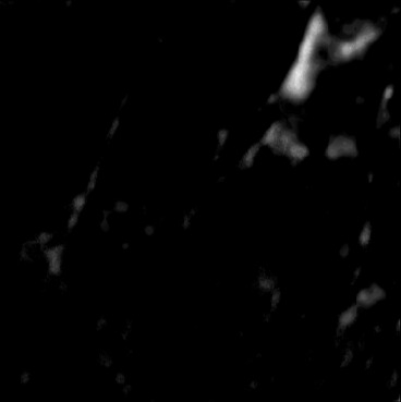 | 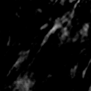 | 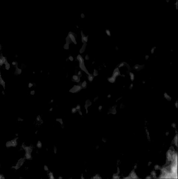 | |
| RMSE | 8.69 | 16.16 | 10.87 | 15.78 | 13.57 | 17.49 | 34.35 | 21.25 | 28.63 | 20.45 | [m/s] |
| MAE | 4.79 | 7.48 | 6.62 | 8.08 | 7.12 | 13.58 | 26.08 | 15.02 | 22.64 | 15.84 | [m/s] |
| SSIM | 0.88 | 0.91 | 0.84 | 0.88 | 0.89 | 0.76 | 0.73 | 0.66 | 0.70 | 0.74 |
Ellipsoids Setup
In the quantitative evaluation, the network converges to average RMSE, MAE, and MAPE of (mean SD), and %, respectively (over 10 runs). SD is the standard deviation value. The typical RMSE for these kinds of simulated datasets tested on encoder-decoder networks are reported in the range (Feigin et al., 2019) and (Oh et al., 2021).
Figure 5, green box, shows that the network can handle cases with single and separated multiple lesions (Cases 1, 2, and 3), overlapping lesions (Cases 4 and 5), and lesions placed partially inside another lesion (Case 2). As the number of inclusions and the complexity of the medium increases the corresponding error rates increase. A deviation from the GT is present in all cases at the boundary of the lesion and background medium which can be seen as line distortions in the boundaries (Cases 1, 2, and 3) and brighter regions in absolute difference images (Cases 1, 2, 4 and 5). Note that for easier visual interpretation of SoS difference at the edges, only in absolute difference figures, errors lower than are excluded (Feigin et al., 2019). The network is more likely to over/underestimate values when the lesion is placed in the shadow of another lesion or in the case of overlapping lesions (Cases 4, 2, and 5).
T2US Setup
The network trained with T2US dataset converges to average RMSE, MAE and MAPE of , and %, respectively, over 10 runs (Table 1). Although these error rates are higher compared to the aforementioned Ellipsoids setup, they are still relevant, since they are in the range of the RMSE values reported by other groups that used simulated data for training (RMSE of (Feigin et al., 2019) and (Oh et al., 2021)).
Figure 5, blue box, demonstrates qualitative results. The network can handle the gradual variation in the medium even when the boundaries are not clear (Cases 7 and 10). Additionally, the network can reconstruct some of the fine structures (Cases 6 and 8). However, in some cases, when the variation between the SoS values for the fine structures and the background is low some of the fine structures are missed by the network (Cases 7 and 9).
Combined Setup
First of all, we tested the trained networks with their dissimilar test set, meaning, the network trained on the Ellipsoids setup is tested on the T2US test set, and the network trained on the T2US setup is tested on the Ellipsoids test set. Although networks trained with each set of simulated data were capable of performing well on their corresponding test dataset, testing them using the dissimilar test set resulted in failure and high RMSE and MAE values shown in Table 2. Therefore, as expected the network only generalizes on the same distribution on which it is trained.
| RMSE () | Ellipsoids (train) | T2US (train) |
| Ellipsoids (test) | ||
| T2US (test) | ||
| MAE () | Ellipsoids (train) | T2US (train) |
| Ellipsoids (test) | ||
| T2US (test) |
The aim of the study is to improve the performance and stability of the existing approach by including more complicated, tissue-like structures. Therefore, both sets are needed to be presented to the network during the training phase. We have chosen a multi-task learning approach to train the network on both datasets jointly. Multi-task learning is an approach where the data from task A and task B are interleaved so the weights can be jointly optimized (Kirkpatrick et al., 2017).
The test dataset as well as the training dataset is a half-half combination of Ellipsoids and T2US setups. Using the Combined dataset as shown in Table 1, the network converges to mean RMSE of , MAE of and MAPE of % (over 10 runs). The error rates infer that the network is jointly optimized on both datasets and is capable of performing on both data representations.
Figure 5, red box, shows 10 predictions from the network trained with the Combined setup. For the shown cases in Figure 5, some of the cases show improvements (Cases 3, 5, 6, and 8) but on average, in comparison to singles sets, the errors are slightly higher when trained on the Combined setup. Nevertheless, the network can still handle multiple inclusions (Cases 2, 3, and 5), overlapping inclusions (Cases 2, 4, and 5), gradual variations (Cases 7 and 10) and even reconstruct fine structures (Case 6).
Clinical Relevance
Based on the study by Li et al. (2009), fatty tissue and breast parenchyma have mean SoS values of and , respectively. Whereas the mean SoS for lesions is higher, e.g., for malignant breast lesions the mean value is , and for benign lesions is . Ruby et al. (2019) demonstrated that breast lesions create SoS contrast (SoS) compared to the background tissue. They reported SoS in range and m/s for malignant and benign lesions, respectively. Malignant lesions show significantly higher SoS compared to benign lesions . Therefore, theoretically, the achieved error measured shown in Table 1 are clinically relevant.
4.1.2 Out-of-Domain Data
In section 4.1.1, we showed that the network trained with the Combined dataset can learn both representations. Nevertheless, the network can be sensitive to the variation of acoustic parameters, e.g., echogenicity, the density of the scatterers, noise, and geometry. A comprehensive analysis of the sensitivity of the network to these parameters is currently missing from the literature that can provide insights to improve the quality of the simulated training data for future studies. Additionally, we argue that the diverse training set, i.e., combining the baseline dataset (Ellipsoids setup) with our proposed setup (T2US) improves the stability of the network. Thus, in this section, we test the networks trained with the Ellipsoids dataset and the Combined dataset on simulated test sets that have different properties compared to the training dataset, e.g., echogenicity, the density of reflective scatterers, noise characteristics, and geometry.
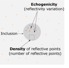
An example of a simulation medium is shown in Figure 6. Consider a medium with a homogeneous background with scatterers randomly distributed inside the medium. Different echogenicities can be created by increasing or decreasing the impedance contrast of the small scatterers or speckles included in the heterogeneity (pink and red dots inside the inclusion in Figure 6). The anechoic region can be modeled by removing the speckles inside the inclusion. The following properties are kept constant through the simulation of the training sets: (i) Echogenicity: only hyperechogenic regions are modeled (by using speckles with a higher standard deviation (i.e., more echoic) than the background for % of the scatterers). (ii) Density of scatterers: the number of scatterers shown as ’Density of reflective points’ in Figure 6 is kept constant and equal to % of the grid points for all training sets. In the following section, these parameters are altered to investigate the stability of the trained networks.
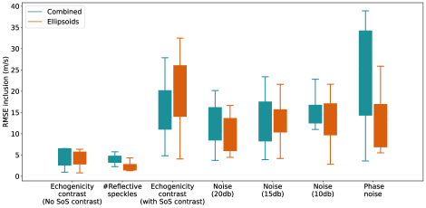
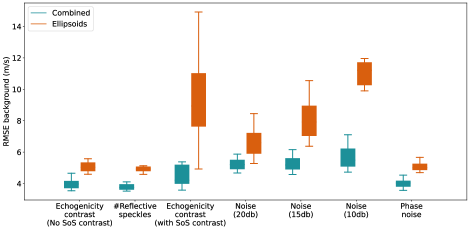
For out-of-domain test sets we simulated a simple homogeneous medium with an inclusion placed in the central section of the medium but introduced variations in echogenicity, the number of reflective scatters, noise compared to the training set, and computed RMSE of two networks inside the inclusion area and in the background. The results are presented in Figure 7. Example cases of each variation scenario are shown in Figure 8, Figure 9 and Figure 10 for quantitative evaluations.
Echogenicity and Speckles
| Case 1 | Case 2 | Case 3 | Case 4 | Case 5 | Case 6 | Case 7 | Case 8 | ||
| B-mode |  |  |  | 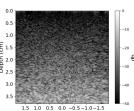 |  |  | 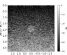 |  | |
| GT |  | 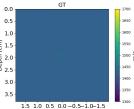 |  |  |  |  |  |  | |
| PredictedSoSCombined |  |  |  |  |  |  |  |  | |
| AbsoluteDifference | 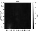 |  |  |  |  |  |  |  | |
| PredictedSoSEllipsoids |  |  |  |  |  |  |  |  | |
| AbsoluteDifference |  |  |  |  |  |  | 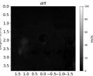 |  |
Number of Reflective Speckles (Case 8): Case 8 similar to Case 4 shows an isoechoic region but Case 8 has the double number of reflective speckles inside the inclusion area; nevertheless the number of reflective speckles does not affect the indication of inclusion area in the figure.
Echogenicity Contrast without SoS Contrast
The aim of this investigation is to demonstrate that the networks are only sensitive to SoS variations, thus, the presence of inclusions in the b-mode images (created by echogenicity contrast) does not necessarily indicate SoS contrast. As a result, the network is not supposed to show any SoS contrast in the predictions.
In Figure 7, Echogenicity contrast (No SoS contrast) boxes show the RMSE values inside the inclusion and in the background for 20 cases where there is an inclusion present in the medium but the inclusion only has an echogenicity contrast and the SoS value inside the inclusion is same as the background. For instance, Figure 8, Case 1-7 shows examples of such setup, homogeneous mediums with anechoic, hypoechoic, isoechoic, and hyperechoic inclusions with no SoS contrast.
Based on Figure 7, both networks show comparable RMSE inside the inclusions. The RMSE of the background is higher for the Ellipsoids setup compared to the Combined setup. Qualitatively, this can be seen as more over/underestimations in the background region in Figure 8, e.g., Cases 2, 3, and 4.
Nevertheless, both networks despite the presence of inclusion with echogenicity contrast, due to lack of SoS contrast, as expected, do not predict any inclusion-shaped area in the SoS domain. This investigation shows that the network learns the SoS reconstruction.
Number of Reflective Speckles
To the best of our knowledge, currently there is no reference method available to determine the optimum numbers of scatterers for training data generation. Thus, the aim of this investigation is to evaluate the sensitivity of the network to the number of scatterers modeled in the heterogeneity.
Figure 7 #Reflective speckle boxes demonstrate the RMSE values for 20 cases where the number of scatterers varies from % to % of grid points with the step of %. Figure 8, Case 8 shows an example where the number of scatterers increased from % to %.
Based on Figure 7, for 20 cases, the RMSE of the Combined network inside the inclusion has a similar distribution but is slightly higher than the RMSE of the Ellipsoids setup. On the other hand, the RMSE of the Combined network for the background region is lower than the Ellipsoids network. For none of the evaluated cases (similar to Figure 8, Case 8) modifying the number of scatterers did not affect the network predictions regarding the presence of an inclusion. Consequently, varied numbers of scatterers can be modeled for the simulation of the training data.
| Case 1 | Case 2 | Case 3 | Case 4 | Case 5 | Case 6 | Case 7 | Case 8 | ||
| B-mode | 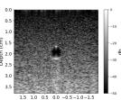 |  | 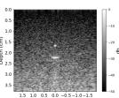 | 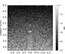 |  |  |  |  | |
| GT |  |  |  |  |  |  |  |  | |
| PredictedSoSCombined | 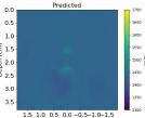 | 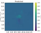 | 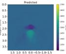 | 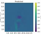 |  |  |  |  | |
| AbsoluteDifference | 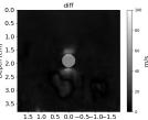 |  | 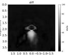 | 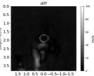 |  | 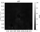 |  | 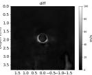 | |
| PredictedSoSEllipsoids | 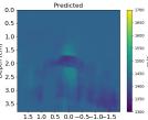 | 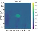 | 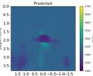 |  | 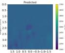 | 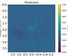 | 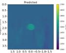 |  | |
| AbsoluteDifference | 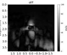 | 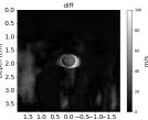 | 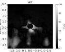 | 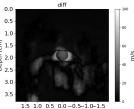 | 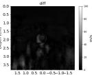 | 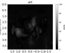 | 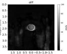 | 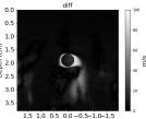 |
| Case 1 | Case 2 | Case 3 | Case 4 | Case 5 | Case 6 | Case 7 | Case 8 | ||
| B-mode |  |  | 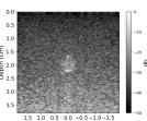 |  |  |  |  | 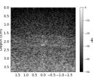 | |
| GT | 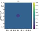 |  |  |  |  |  |  |  | |
| PredictedSoSCombined | 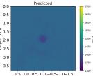 |  | 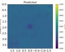 |  | 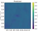 | 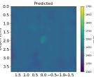 | 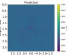 |  | |
| AbsoluteDifference | 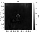 | 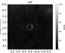 |  | 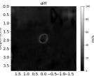 | 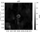 | 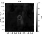 | 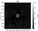 | 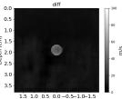 | |
| PredictedSoSEllipsoids | 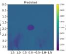 |  | 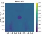 | 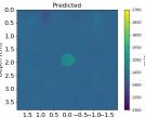 | 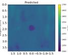 |  |  |  | |
| AbsoluteDifference | 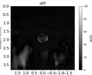 | 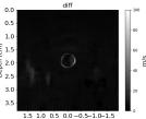 | 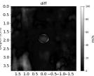 | 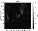 | 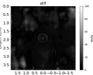 | 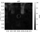 | 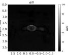 | 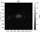 |
Echogenicity Contrast with SoS Contrast
Since in the training set we only considered hyperechoic regions, the aim of this investigation is to show how the networks behave in cases with SoS contrast with varied echogenicity characteristics.
Figure 7 Echogenicity contrast (with SoS contrast), compares the RMSE values inside the inclusion and in the background for 20 cases with SoS contrast in the range with step, where is the SoS in the background. For these sets, the Combined setup outperforms the Ellipsoids setup both inside the inclusion and in the background region.
Figure 9 shows anechoic and isoechoic inclusions with SoS contrast from the background. Cases 1 and 2, the anechoic inclusions, have SoS contrast from the background. Cases 3-8 show SoS contrast in range with steps.
Generally, the RMSE values are higher compared to the previous cases shown in Figure 7 Echogenicity contrast (No SoS contrast) and #Reflective speckles. This can be seen in Figure 9 absolute difference images. Anechoic inclusions are more challenging due to the absence of scatterers inside the inclusions. For isoechoic cases, the predicted SoS maps by the Combined setup have clearer margins and fewer under/overestimations outside the inclusion. Additionally, a shadowing effect can be seen directly below the inclusion which increases the overall RMSE.
The interesting finding from this investigation is that the networks can indicate the presence of inclusion even when the inclusion is not visible in the b-mode images (isoechoic cases). Although isoechoic lesions are often benign, they are known to be challenging to find in conventional ultrasound imaging, and often a complementary tool is required to find those lesions (Kim et al., 2011). SoS reconstruction can be a potential solution to find these kinds of lesions and prevent false-negative interpretations and a delayed diagnosis of breast cancers.
Noise
The aim of the following sections is to show how additive and phase noise affects the predictions of the networks:
Additive Noise
Additive White Gaussian Noise (AWGN) is added with a target signal-to-noise ratio (SNR) of 10, 15, and 20 db, where . is the power of the signal and is the power of the noise. Figure 7, Noise boxes, show the RMSE comparison inside the inclusion and in the background regions of 20 cases, for each target SNR, with SoS contrast in the range with steps. is the SoS value in the background. For this investigation, only AWGN is added and echogenicity is considered to be hyperechoic (same as the training set).
Based on Figure 7 Noise (20db), Noise (15db), and Noise (10db) boxes, as the additive noise increases, the RMSE values inside the inclusions are increased for both Ellipsoids and Combined setup. However, the variation of the RMSE in the background regions is lower for the Combined setup, and as the noise increases the gap between the two setups increases. This shows that the Combined setup is more robust to the noise. In Figure 10, Cases 3 and 4, and Cases 5 and 6 examples of the data with target SNR of 15 db and 10 db are shown, respectively. Figure 10, Cases 1 and 2 show the original data (without additive noise). The SoS contrast for each pares is of SoS in the background.
Phase Noise
Studies showed that phase distortions can affect SoS predictions (Stähli et al., 2020a; Khun Jush et al., 2021). Therefore, we applied uncorrelated phase distortions by shifting the phase of each channel by a random value in the range radian. Figure 7 Phase noise boxes show the corresponding RMSE values inside the inclusion and for the background in the presence of such a noise for 20 cases. The highest RMSE values and the highest variation between cases for the Combined setup belong to the RMSE inside the inclusions. Figure 10 Cases 7 and 8 show cases with described phase distortions. Although there is an indication of inclusion by both networks, the margins are distorted. Based on Figure 7, the absolute value of the SoS predictions has a higher offset for the Combined setup. This indicates that the Combined setup is highly sensitive to phase distortions.
The predicted SoS values in the background regions for the Combined setup show a similar pattern as Echogenicity contrast (No SoS contrast) and #Reflective speckles where the RMSE is slightly lower than the Ellipsoids setup.
| Case 1 | Case 2 | Case 3 | Case 4 | Case 5 | Case 6 | Case 7 | Case 8 | ||
| B-mode |  | 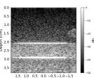 | 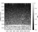 | 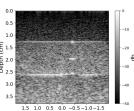 | 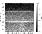 | 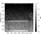 | 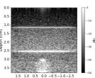 | 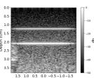 | |
| GT | 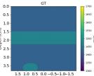 |  | 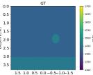 | 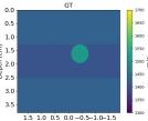 | 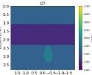 |  | 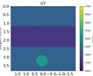 | 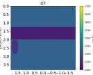 | |
| PredictedSoSCombined | 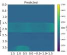 |  | 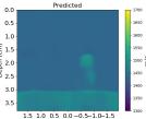 | 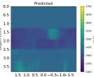 | 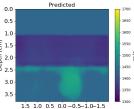 | 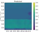 | 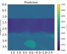 | 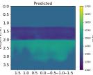 | |
| AbsoluteDifference | 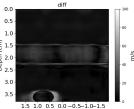 | 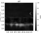 | 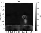 | 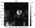 | 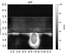 | 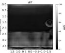 | 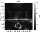 | 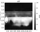 | |
| RMSE | 9.17 | 11.17 | 9.72 | 16.00 | 25.19 | 19.30 | 13.41 | 43.34 | [m/s] |
| PredictedSoSEllipsoids | 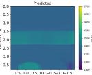 | 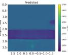 | 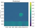 | 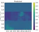 |  | 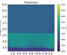 |  | 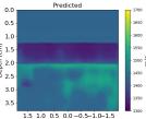 | |
| AbsoluteDifference | 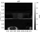 | 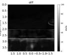 | 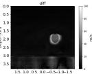 | 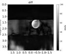 | 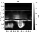 | 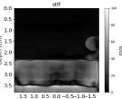 | 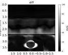 | 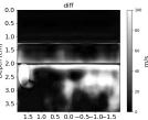 | |
| RMSE | 12.04 | 10.74 | 10.87 | 18.31 | 19.90 | 25.11 | 20.82 | 40.20 | [m/s] |
Layered Phantoms
The aim of this investigation is to demonstrate how the networks behave in the presence of out-of-domain geometry with various echogenicity and SoS contrasts.
We simulated digital phantoms with layered structures and an elliptical inclusion randomly placed inside one of the layers. A layer with a random thickness in the range cm is placed in the medium. The SoS value inside the layer and the inclusions are assigned randomly in the range . The echogenicity of each layer and the inclusion is assigned randomly as well, hence, the layers or/and the inclusions can have echogenicity contrast compared to the training sets.
Figure 11 shows 8 example phantoms. The figure shows that in all cases, the layers could be separated by both networks. Additionally, inclusions independent of their echogenicity are detectable in SoS maps, except for Case 8 for both networks. This case has an inclusion that is only partially in the field of view. Since a single PW is used, it is expected that with increasing the depth, the performance drops in the sides of the field of view. Case 8 is more challenging because the inclusion is directly below the layer and both networks often under/overestimate the SoS values directly below the layer. Similar observations can be found in Figure11 Cases 2, 5, and 7.
We created 500 cases of layered phantoms, the average RMSE of 500 cases for the Combined network is with a standard deviation of and for the Ellipsoids network, the average RMSE is with a standard deviation of . The average RMSE for both networks is in a similar range as the RMSE of T2US and Combined setup but the standard deviation is higher. This indicates that it is probable that cases similar to e.g., Figure 11 Case 8 appear where an over/underestimation artifact is present directly below the layer structures. Nevertheless, in most cases, the margins and inclusions are detected correctly. Thus, although the training data does not include layer-like structures the network can handle out-of-domain geometry with any given echogenicity.
4.2 Experimental Data
4.2.1 Single Frame
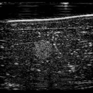
In this section, we test the trained networks on a dataset acquired from the CIRS multi-modality breast phantom. The phantom consists of an anechoic skin layer on top (directly below the transducer). Directly below the skin layer is the breast tissue mimicking layer with hyperechoic characteristics with randomly mixed embedded fibers. Hereafter, we will refer to this layer as background tissue. Inside the tissue-mimicking layer, there is an embedded hyperechoic inclusion with SoS contrast from the background layer. We do not have the SoS GT map for this phantom but based on the information provided by the manufacturer the SoS values in this phantom are in the range , where the skin layer has the lower SoS and the inclusion has a higher SoS contrast compared to the background.
| Frame 0 | ||||
 | ||||
| Ellipsoids | T2US | Combined | [m/s] | |
| PredictedSoS | 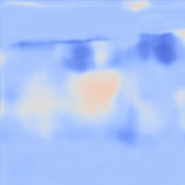 | 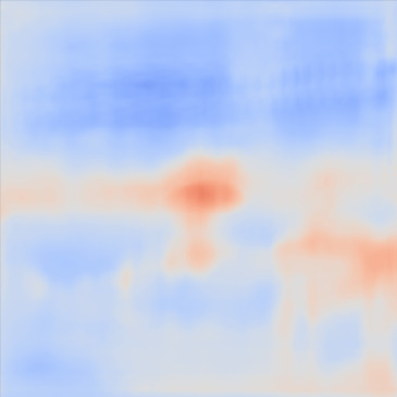 | 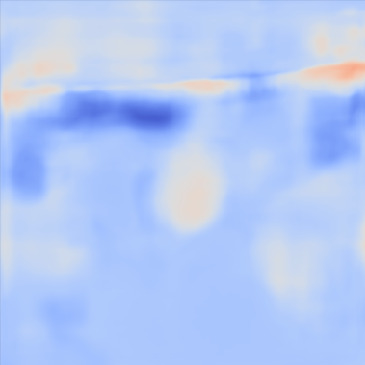 | |
| Overlayimage | 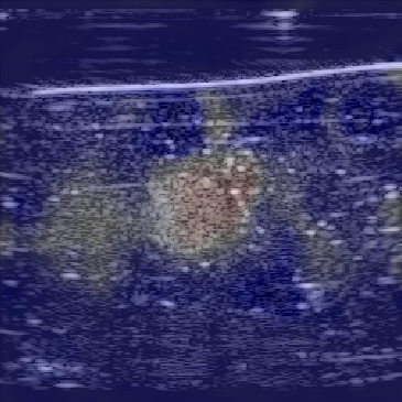 | 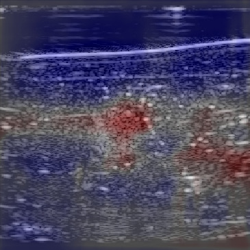 | 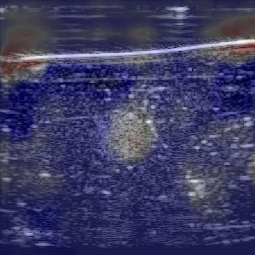 |
Figure 12 shows the predicted SoS values for all three setups. Since the exact SoS GT is not available, from this point on we are going to use the relative SoS values to compare the results:
- (i)
The predicted SoS values are in the expected range (except for the artifact directly below the skin layer, this effect was observed in layered structured digital phantoms as well).
- (ii)
The Ellipsoids and the Combined setups were capable of separating the skin margin from the background tissue, whereas the T2US setup fails to find the skin layer correctly.
- (iii)
The inclusions are separated with higher SoS values compared to the background for all three setups. The margins of the inclusion are best detected by the Combined setup and second best by the Ellipsoids setup but there are several artifacts present in the predicted maps using T2US setup. Although this setup worked well on the simulated data, it is too sensitive to the highly reflective scatterers embedded in the phantom when tested on measured data. Due to the high sensitivity, we removed this setup from the robustness investigation for consecutive frames presented in the next section.
4.2.2 Consecutive Frames
| Frame 1 | Frame 2 | Frame 3 | Frame 4 | Frame 5 | ||
| B-mode | 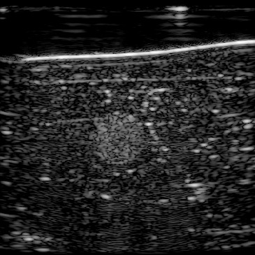 | 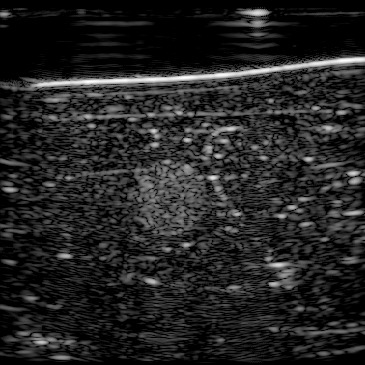 |  | 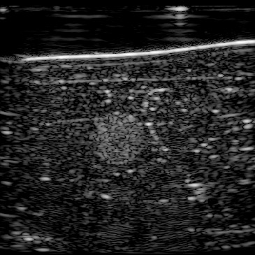 | 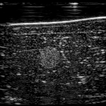 | |
| AbsoluteDifferenceB-mode | 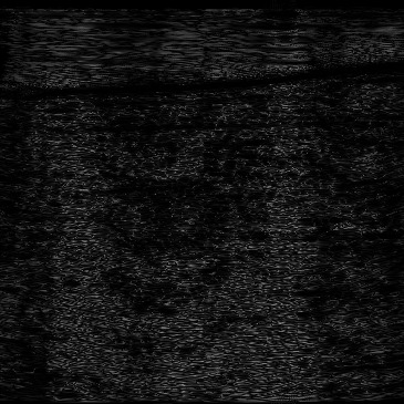 |  |  |  |  | |
| PredictedSoSCombined | 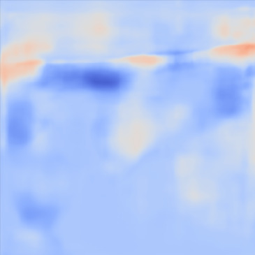 | 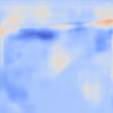 | 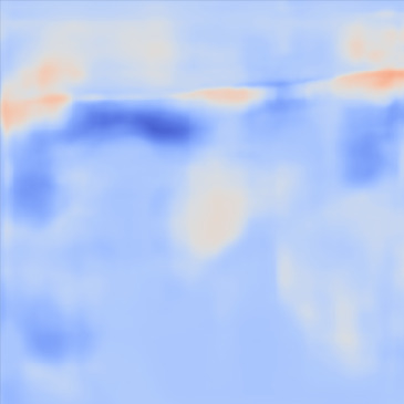 | 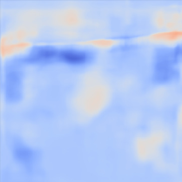 |  | |
| PredictedSoSEllipsoids |  |  |  |  |  |
| Inside Inclusion | Background |
 |  |
| (a) | (b) |
 |  |
| (c) | (d) |
In our previous work (Khun Jush et al., 2020), when tested on the measured data, we realized that the network is sensitive to slight movements during acquisition and electronic noise in the raw data. We mechanically fixed the probe head and phantom to reduce unwanted movements and vibrations during data acquisition and recorded multiple consecutive acquisitions, five of which are shown in Figure 13. Given that the setup is fixed we expect consistent and reproducible predictions for the acquired frames.
Figure 13, 1st row demonstrates the reconstructed b-mode images for 5 frames. We computed the absolute difference of each frame compared to its previous frame which resulted in the image shown in Figure 13, 2nd row. Note that frame 0 is shown in Figure 12, and the difference matrices for frame 1 are computed using frame 0. There is no apparent difference between these frames suggesting phantom movement, thus, the difference is only caused by electrical noise.
In Figure 13, 4th row, the corresponding SoS map of each frame is shown for the network trained on the Ellipsoids dataset alone. Although there are minimum movements between the acquired frames, the inclusion localization margins vary for each frame, thus, the network trained with the Ellipsoids dataset is highly sensitive to the electronic noise.
Figure 13, 3rd row demonstrates the SoS map of each frame for the network trained on the Combined dataset. The variations between predictions from frame to frame are significantly lower than the cases shown in the 3rd row. The variations between frames are mostly present on sides that can possibly be related to the single PW transmission setup. Nevertheless, in comparison, this setup shows lower sensitivity.
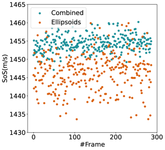
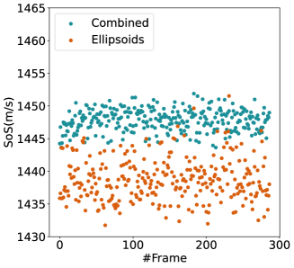
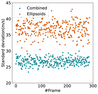
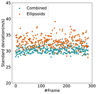
For quantitative comparison, we computed the mean and standard deviation of the predicted SoS maps of 287 consecutive frames of the same view shown in Figure 13. The corresponding scatter plots are shown in Figure 14. The variation between average SoS values inside the inclusion as well as the background shows that for the same field of view, the network trained with the Combined dataset has more consistent predictions. The mean standard deviation for the Combined setup over 287 frames is inside the inclusion and in the background. In comparison, the mean standard deviation for the Ellipsoids setup inside the inclusion is , and in the background is . The overall mean standard deviation of the Combined setup is lower than the Ellipsoids setup which is equal to % improvement. Thereby, mixing the Ellipsoids dataset with the T2US dataset improved the stability of the setup and increased the robustness and reproducibility of the network for consecutive frames.
5 Summary and Conclusion
Deep-learning-based algorithms have predictable run times and therefore have great potential for real-time deployment. However, since they are data-hungry, they pose challenges regarding training data requirements. Particularly, due to the lack of a gold standard method, for SoS reconstruction acquiring real-world data alongside their exact GT sufficient to train these networks is even more challenging. Employing simulated data for training can be advantageous because firstly, it resolves the problem of creating a huge amount of data alongside their exact GT. Secondly, it allows for designing diverse mediums with arbitrary heterogeneous structures and acoustic properties that otherwise would have been time-consuming and costly. In prior studies, a simplified model for tissue modeling was used to create training datasets (Feigin et al., 2019, 2020; Vishnevskiy et al., 2019; Oh et al., 2021).
Transferring deep-learning-based models that are trained on the simulated data to perform robustly on real-world setups is a non-trivial task and models trained on simulated data often only perform well on the same distributions on which they are trained and perform poorly on real setups. In this study, we proposed a new simulation setup for modeling the tissues to reduce the sensitivity and increase the stability of an existing deep-learning-based SoS reconstruction method. Our proposed medium structure is extracted from Tomosynthesis images of breast tissues that are diagnosed with malignant or benign lesions. This setup includes fine, complicated, tissue-like structures. We compared our model with a method that uses artificial ellipsoid structures for modeling organs and tissues introduced by Feigin et al. (2019). Although our proposed model consists of fine and complicated structures, the deep neural network is still able to reconstruct the underlying map and perform well on the simulated data.
Testing each trained network on its dissimilar test dataset demonstrated that neither the training dataset based on artificial ellipsoids structures nor the training dataset derived from Tomosynthesis data contains sufficient diversified information to generalize the learning of the network. Hence, we mixed two datasets and investigated the possibility of training the network jointly with both data representations. The network is capable of learning both sets at once.
Additionally, in the Out-of-Domain section, we addressed the echogenicity characteristics of the simulated mediums and compared the performance of the networks with out-of-domain echogenicity, scatterers, medium structures, and noise presence for simulated data. Both networks can handle various echogenicity and different densities of scatterers. However, for the Ellipsoids setup varying these properties results in over/underestimations, especially in the background regions which can lead to false positives. We showed that the network can detect SoS contrast even when no inclusion is visible in b-mode images. In the presence of noise, the network trained with the Combined dataset outperforms the Ellipsoids setup. The gap increases by increasing the noise. In the presence of phase noise, both networks showed high error rates and inconsistent predictions that show the sensitivity of the networks to phase distortions.
In the setup with measured data, all models could localize the embedded inclusion inside the tissue-mimicking phantom but the estimated SoS maps of the network trained with the Combined dataset, have cleaner margins and fewer misestimations.
Furthermore, we tested the performance of the networks in terms of reproducibility and stability on consecutive frames of the same field of view over 287 frames and demonstrated that by mixing the training datasets we could improve the stability of the network by 18%.
We conclude two points; firstly, compared to the baseline training data generation method proposed by Feigin et al. (2019), our proposed method improves the overall performance of the network both on simulated and measured data setup (especially in the presence of noise) by using diverse simulated dataset. Secondly, the investigations on the out-of-domain simulated data showed that the number of the scatterers and the echogenicity of the simulation has the least impact on the stability of the network, whereas, the network is highly sensitive to phase noises. This should be taken into account in the postprocessing and filtering steps of the ultrasound RF data. Avoiding phase distortions is the key to creating a robust setup.
The investigated method has great potential and is advantageous because first of all it is based on a pulse-echo setup, thus, does not require special hardware and can be used with handheld probes. Secondly, it only requires a single PW acquisition which makes it easy to create simulated data to integrate deep neural networks. The biggest advantage of employing deep neural networks is that they can be used in real-time during inference. Plus, a diverse dataset that covers a wide range of shapes, SoS values, and acoustic properties eliminates the burden of hyperparameter tuning and prior assumptions often required by the analytical and optimization methods.
6 Limitations and Future Research
Despite encouraging initial results, the proposed method has the following limitations that can be considered for future works. Firstly, there still remains the challenge of quantifying the error on measured data for these setups. Currently, the exact GT for our measured data is not available. Nevertheless, the accuracy of the predicted SoS values can be evaluated by using ultrasound tomography devices. In ultrasound tomography, due to multi-sided access to the tissues, it is possible to calculate the SoS values of the tissues under examination using Time-of-Flight (ToF). Thus, using this approach the expected range of the SoS values can be determined and consequently the accuracy of the predicted values in the pulse-echo setup can be evaluated in comparison. It is noteworthy that the effectiveness of SoS methods (using ultrasound tomography or pulse-echo setup) for clinical integration is still in the research phase.
Secondly, although the new proposed setup improved the performance of the deep neural network under investigation, further research can focus on designing more generalized simulation setups: e.g., the presented setup is a 2D model, and therefore off-axis reflections from the z-direction are not modeled due to high computational effort and memory requirements. Thus, one idea would be to investigate 3D modeling and its effect on the stability of the network. Another approach can include prior knowledge about the tissue type present in Tomosynthesis images by accurately segmenting and annotating the images and mapping the intensity values to the expected SoS values of the corresponding tissue types. In general, despite extensive research, developing models that represent realistic tissue structures poses many challenges due to the complex structure and mechanical response of soft tissues. For deep learning approaches the characteristics of the measurement devices affect the network generalization to a great extent and therefore, should be taken into account. This further complicates the problem, instead, employing domain adaptation techniques can be a possible solution to bridge the gap between simulated and measured data, an example of such a solution for beamforming is examined by Tierney et al. (2021).
Acknowledgments
We thank Prof. Michael Golatta and the university hospital of Heidelberg for providing the Tomosynthesis dataset.
Ethical Standards
The work follows appropriate ethical standards in conducting research and writing the manuscript, following all applicable laws and regulations regarding the treatment of animals or human subjects.
Disclaimer
The information in this paper is based on research results that are not commercially available.
References
- Agrawal et al. (2021) Sumit Agrawal, Thaarakh Suresh, Ankit Garikipati, Ajay Dangi, and Sri-Rajasekhar Kothapalli. Modeling combined ultrasound and photoacoustic imaging: Simulations aiding device development and artificial intelligence. Photoacoustics, 24:100304, 2021.
- Agudo et al. (2018) O Calderon Agudo, Lluis Guasch, Peter Huthwaite, and Michael Warner. 3d imaging of the breast using full-waveform inversion. In Proc. Int. Workshop Med. Ultrasound Tomogr., pages 99–110, 2018.
- Benjamin et al. (2018) Alex Benjamin, Rebecca E Zubajlo, Manish Dhyani, Anthony E Samir, Kai E Thomenius, Joseph R Grajo, and Brian W Anthony. Surgery for obesity and related diseases: I. a novel approach to the quantification of the longitudinal speed of sound and its potential for tissue characterization. Ultrasound in medicine & biology, 44(12):2739–2748, 2018.
- Bernhardt et al. (2020) Melanie Bernhardt, Valery Vishnevskiy, Richard Rau, and Orcun Goksel. Training variational networks with multidomain simulations: Speed-of-sound image reconstruction. IEEE Transactions on Ultrasonics, Ferroelectrics, and Frequency Control, 67(12):2584–2594, 2020.
- Blickstein et al. (1995) Isaac Blickstein, Reinaldo Goldchmit, Selwyn D Strano, Ran D Goldman, and Naftali Barzili. Echogenicity of fibroadenoma and carcinoma of the breast. quantitative comparison using gain-assisted densitometric evaluation of sonograms. Journal of ultrasound in medicine, 14(9):661–664, 1995.
- Carra et al. (2014) Bradley J Carra, Liem T Bui-Mansfield, Seth D O’Brien, and Dillon C Chen. Sonography of musculoskeletal soft-tissue masses: techniques, pearls, and pitfalls. American Journal of Roentgenology, 202(6):1281–1290, 2014.
- Chen et al. (2016) Weifeng Chen, Zhao Fu, Dawei Yang, and Jia Deng. Single-image depth perception in the wild. Advances in neural information processing systems, 29:730–738, 2016.
- Chung and Cho (2015) Hye Won Chung and Kil-Ho Cho. Ultrasonography of soft tissue “oops lesions”. Ultrasonography, 34(3):217, 2015.
- Cong et al. (2013) Weijian Cong, Jian Yang, Yue Liu, and Yongtian Wang. Fast and automatic ultrasound simulation from ct images. Computational and mathematical methods in medicine, 2013, 2013.
- Dillenseger et al. (2009) Jean-Louis Dillenseger, Soizic Laguitton, and Éric Delabrousse. Fast simulation of ultrasound images from a ct volume. Computers in biology and medicine, 39(2):180–186, 2009.
- Duric et al. (2007) Nebojsa Duric, Peter Littrup, Lou Poulo, Alex Babkin, Roman Pevzner, Earle Holsapple, Olsi Rama, and Carri Glide. Detection of breast cancer with ultrasound tomography: First results with the computed ultrasound risk evaluation (cure) prototype. Medical physics, 34(2):773–785, 2007.
- Eigen and Fergus (2015) David Eigen and Rob Fergus. Predicting depth, surface normals and semantic labels with a common multi-scale convolutional architecture. In Proceedings of the IEEE international conference on computer vision, pages 2650–2658, 2015.
- Feigin et al. (2019) Micha Feigin, Daniel Freedman, and Brian W Anthony. A deep learning framework for single-sided sound speed inversion in medical ultrasound. IEEE Transactions on Biomedical Engineering, 67(4):1142–1151, 2019.
- Feigin et al. (2020) Micha Feigin, Manuel Zwecker, Daniel Freedman, and Brian W Anthony. Detecting muscle activation using ultrasound speed of sound inversion with deep learning. In 2020 42nd Annual International Conference of the IEEE Engineering in Medicine & Biology Society (EMBC), pages 2092–2095. IEEE, 2020.
- Gao et al. (2019) Zhifan Gao, Sitong Wu, Zhi Liu, Jianwen Luo, Heye Zhang, Mingming Gong, and Shuo Li. Learning the implicit strain reconstruction in ultrasound elastography using privileged information. Medical image analysis, 58:101534, 2019.
- Garcia et al. (2013) Damien Garcia, Louis Le Tarnec, Stéphan Muth, Emmanuel Montagnon, Jonathan Porée, and Guy Cloutier. Stolt’s fk migration for plane wave ultrasound imaging. IEEE transactions on ultrasonics, ferroelectrics, and frequency control, 60(9):1853–1867, 2013.
- Gasse et al. (2017) Maxime Gasse, Fabien Millioz, Emmanuel Roux, Damien Garcia, Hervé Liebgott, and Denis Friboulet. High-quality plane wave compounding using convolutional neural networks. IEEE transactions on ultrasonics, ferroelectrics, and frequency control, 64(10):1637–1639, 2017.
- Gemmeke and Ruiter (2007) H Gemmeke and NV Ruiter. 3d ultrasound computer tomography for medical imaging. Nuclear Instruments and Methods in Physics Research Section A: Accelerators, Spectrometers, Detectors and Associated Equipment, 580(2):1057–1065, 2007.
- Glorot and Bengio (2010) Xavier Glorot and Yoshua Bengio. Understanding the difficulty of training deep feedforward neural networks. In Proceedings of the thirteenth international conference on artificial intelligence and statistics, pages 249–256. JMLR Workshop and Conference Proceedings, 2010.
- Gokhale (2009) Sudheer Gokhale. Ultrasound characterization of breast masses. The Indian journal of radiology & imaging, 19(3):242, 2009.
- Goyal and Bengio (2020) Anirudh Goyal and Yoshua Bengio. Inductive biases for deep learning of higher-level cognition. arXiv preprint arXiv:2011.15091, 2020.
- Gyöngy and Kollár (2015) Miklós Gyöngy and Sára Kollár. Variation of ultrasound image lateral spectrum with assumed speed of sound and true scatterer density. Ultrasonics, 56:370–380, 2015.
- Hachiya et al. (1994) Hiroyuki Hachiya, Shigeo Ohtsuki, and Motonao Tanaka. Relationship between speed of sound in and density of normal and diseased rat livers. Japanese journal of applied physics, 33(5S):3130, 1994.
- Hager et al. (2019) Pascal A Hager, Farnaz Kuhn Jush, Markus Biele, Peter M Düppenbecker, Oliver Schmidt, and Luca Benini. Lightabvs: A digital ultrasound transducer for multi-modality automated breast volume scanning. In 2019 IEEE International Ultrasonics Symposium (IUS), 2019.
- Heller and Schmitz (2021) Marvin Heller and Georg Schmitz. Deep learning-based speed-of-sound reconstruction for single-sided pulse-echo ultrasound using a coherency measure as input feature. In 2021 IEEE International Ultrasonics Symposium (IUS), pages 1–4. IEEE, 2021.
- Hoerig et al. (2018) Cameron Hoerig, Jamshid Ghaboussi, and Michael F Insana. Data-driven elasticity imaging using cartesian neural network constitutive models and the autoprogressive method. IEEE transactions on medical imaging, 38(5):1150–1160, 2018.
- Huang and Li (2004) Sheng-Wen Huang and Pai-Chi Li. Experimental investigation of computed tomography sound velocity reconstruction using incomplete data. IEEE transactions on ultrasonics, ferroelectrics, and frequency control, 51(9):1072–1081, 2004.
- Javaherian et al. (2020) Ashkan Javaherian, Felix Lucka, and Ben T Cox. Refraction-corrected ray-based inversion for three-dimensional ultrasound tomography of the breast. Inverse Problems, 36(12):125010, 2020.
- Jensen et al. (2016) Jonas Jensen, Matthias Bo Stuart, and Jørgen Arendt Jensen. Optimized plane wave imaging for fast and high-quality ultrasound imaging. IEEE transactions on ultrasonics, ferroelectrics, and frequency control, 63(11):1922–1934, 2016.
- Jirik et al. (2012) Radovan Jirik, Igor Peterlik, Nicole Ruiter, Jan Fousek, Robin Dapp, Michael Zapf, and Jiri Jan. Sound-speed image reconstruction in sparse-aperture 3-d ultrasound transmission tomography. IEEE transactions on ultrasonics, ferroelectrics, and frequency control, 59(2):254–264, 2012.
- Khodr et al. (2015) Zeina G Khodr, Mark A Sak, Ruth M Pfeiffer, Nebojsa Duric, Peter Littrup, Lisa Bey-Knight, Haythem Ali, Patricia Vallieres, Mark E Sherman, and Gretchen L Gierach. Determinants of the reliability of ultrasound tomography sound speed estimates as a surrogate for volumetric breast density. Medical physics, 42(10):5671–5678, 2015.
- Khun Jush et al. (2020) Farnaz Khun Jush, Markus Biele, Peter Michael Dueppenbecker, Oliver Schmidt, and Andreas Maier. Dnn-based speed-of-sound reconstruction for automated breast ultrasound. In 2020 IEEE International Ultrasonics Symposium (IUS), pages 1–7. IEEE, 2020.
- Khun Jush et al. (2021) Farnaz Khun Jush, Peter Michael Dueppenbecker, and Andreas Maier. Data-driven speed-of-sound reconstruction for medical ultrasound: Impacts of training data format and imperfections on convergence. In Annual Conference on Medical Image Understanding and Analysis, pages 140–150. Springer, 2021.
- Kim et al. (2011) Min Jung Kim, Ji Youn Kim, Jung Hyun Yoon, Ji Hyun Youk, Hee Jung Moon, Eun Ju Son, Jin Young Kwak, and Eun-Kyung Kim. How to find an isoechoic lesion with breast us. Radiographics, 31(3):663–676, 2011.
- Kirkpatrick et al. (2017) James Kirkpatrick, Razvan Pascanu, Neil Rabinowitz, Joel Veness, Guillaume Desjardins, Andrei A Rusu, Kieran Milan, John Quan, Tiago Ramalho, Agnieszka Grabska-Barwinska, et al. Overcoming catastrophic forgetting in neural networks. Proceedings of the national academy of sciences, 114(13):3521–3526, 2017.
- Kutter et al. (2009) Oliver Kutter, Ramtin Shams, and Nassir Navab. Visualization and gpu-accelerated simulation of medical ultrasound from ct images. Computer methods and programs in biomedicine, 94(3):250–266, 2009.
- Laina et al. (2016) Iro Laina, Christian Rupprecht, Vasileios Belagiannis, Federico Tombari, and Nassir Navab. Deeper depth prediction with fully convolutional residual networks. In 2016 Fourth international conference on 3D vision (3DV), pages 239–248. IEEE, 2016.
- Lee et al. (2017) June-Goo Lee, Sanghoon Jun, Young-Won Cho, Hyunna Lee, Guk Bae Kim, Joon Beom Seo, and Namkug Kim. Deep learning in medical imaging: general overview. Korean journal of radiology, 18(4):570–584, 2017.
- Li et al. (2009) Cuiping Li, Nebojsa Duric, Peter Littrup, and Lianjie Huang. In vivo breast sound-speed imaging with ultrasound tomography. Ultrasound in medicine & biology, 35(10):1615–1628, 2009.
- Li et al. (2014) Cuiping Li, Gursharan S Sandhu, Olivier Roy, Neb Duric, Veerendra Allada, and Steven Schmidt. Toward a practical ultrasound waveform tomography algorithm for improving breast imaging. In Medical Imaging 2014: Ultrasonic Imaging and Tomography, volume 9040, pages 445–454. SPIE, 2014.
- Li et al. (2010) Shengying Li, Marcel Jackowski, Donald P Dione, Trond Varslot, Lawrence H Staib, and Klaus Mueller. Refraction corrected transmission ultrasound computed tomography for application in breast imaging. Medical physics, 37(5):2233–2246, 2010.
- Linda et al. (2011) Anna Linda, Chiara Zuiani, Michele Lorenzon, Alessandro Furlan, Rossano Girometti, Viviana Londero, and Massimo Bazzocchi. Hyperechoic lesions of the breast: not always benign. American Journal of Roentgenology, 196(5):1219–1224, 2011.
- Lucka et al. (2021) Felix Lucka, Mailyn Pérez-Liva, Bradley E Treeby, and Ben T Cox. High resolution 3d ultrasonic breast imaging by time-domain full waveform inversion. Inverse Problems, 38(2):025008, 2021.
- Lundervold and Lundervold (2019) Alexander Selvikvåg Lundervold and Arvid Lundervold. An overview of deep learning in medical imaging focusing on mri. Zeitschrift für Medizinische Physik, 29(2):102–127, 2019.
- Maier et al. (2019) Andreas Maier, Christopher Syben, Tobias Lasser, and Christian Riess. A gentle introduction to deep learning in medical image processing. Zeitschrift für Medizinische Physik, 29(2):86–101, 2019.
- Mainak et al. (2019) Biswas Mainak, Kuppili Venkatanareshbabu, Saba Luca, Reddy Edla Damodar, Cuadrado-Godia Elisa, Marinhoe Rui Tato, Nicolaides Andrew, et al. State-of-the-art review on deep learning in medical imaging. Frontiers in Bioscience-Landmark, 24(3):380–406, 2019.
- Malik et al. (2018) Bilal Malik, Robin Terry, James Wiskin, and Mark Lenox. Quantitative transmission ultrasound tomography: Imaging and performance characteristics. Medical physics, 45(7):3063–3075, 2018.
- Martin et al. (2019) Eleanor Martin, Jiri Jaros, and Bradley E Treeby. Experimental validation of k-wave: Nonlinear wave propagation in layered, absorbing fluid media. IEEE transactions on ultrasonics, ferroelectrics, and frequency control, 67(1):81–91, 2019.
- Mischi et al. (2020) Massimo Mischi, Muyinatu A Lediju Bell, Ruud JG van Sloun, and Yonina C Eldar. Deep learning in medical ultrasound—from image formation to image analysis. IEEE Transactions on Ultrasonics, Ferroelectrics, and Frequency Control, 67(12):2477–2480, 2020.
- Mohammadi et al. (2021) Narges Mohammadi, Marvin M Doyley, and Mujdat Cetin. Ultrasound elasticity imaging using physics-based models and learning-based plug-and-play priors. In ICASSP 2021-2021 IEEE International Conference on Acoustics, Speech and Signal Processing (ICASSP), pages 1165–1169. IEEE, 2021.
- Oh et al. (2021) SeokHwan Oh, Myeong-Gee Kim, Youngmin Kim, Hyuksool Kwon, and Hyeon-Min Bae. A neural framework for multi-variable lesion quantification through b-mode style transfer. In International Conference on Medical Image Computing and Computer-Assisted Intervention, pages 222–231. Springer, 2021.
- Opieliński et al. (2018) Krzysztof J Opieliński, Piotr Pruchnicki, Paweł Szymanowski, Wioletta K Szepieniec, Hanna Szweda, Elżbieta Świś, Marcin Jóźwik, Michał Tenderenda, and Mariusz Bułkowski. Multimodal ultrasound computer-assisted tomography: An approach to the recognition of breast lesions. Computerized Medical Imaging and Graphics, 65:102–114, 2018.
- Pérez-Liva et al. (2017) M Pérez-Liva, JL Herraiz, JM Udías, E Miller, BT Cox, and BE Treeby. Time domain reconstruction of sound speed and attenuation in ultrasound computed tomography using full wave inversion. The Journal of the Acoustical Society of America, 141(3):1595–1604, 2017.
- Qu et al. (2012) Xiaolei Qu, Takashi Azuma, Jack T Liang, and Yoshikazu Nakajima. Average sound speed estimation using speckle analysis of medical ultrasound data. International journal of computer assisted radiology and surgery, 7(6):891–899, 2012.
- Ramani et al. (2021) SK Ramani, Ashita Rastogi, Nita Nair, Tanuja M Shet, and Meenakshi H Thakur. Hyperechoic lesions on breast ultrasound: All things bright and beautiful? Indian Journal of Radiology and Imaging, 2021.
- Roy et al. (2010) Olivier Roy, I Jovanović, Ali Hormati, Reza Parhizkar, and Martin Vetterli. Sound speed estimation using wave-based ultrasound tomography: theory and gpu implementation. In Medical Imaging 2010: Ultrasonic Imaging, Tomography, and Therapy, volume 7629, page 76290J. International Society for Optics and Photonics, 2010.
- Ruby et al. (2019) Lisa Ruby, Sergio J Sanabria, Katharina Martini, Konstantin J Dedes, Denise Vorburger, Ece Oezkan, Thomas Frauenfelder, Orcun Goksel, and Marga B Rominger. Breast cancer assessment with pulse-echo speed of sound ultrasound from intrinsic tissue reflections: Proof-of-concept. Investigative radiology, 54(7):419–427, 2019.
- Sak et al. (2017) Mark Sak, Neb Duric, Peter Littrup, Lisa Bey-Knight, Haythem Ali, Patricia Vallieres, Mark E Sherman, and Gretchen L Gierach. Using speed of sound imaging to characterize breast density. Ultrasound in medicine & biology, 43(1):91–103, 2017.
- Sanabria et al. (2018a) Sergio J Sanabria, Orcun Goksel, Katharina Martini, Serafino Forte, Thomas Frauenfelder, Rahel A Kubik-Huch, and Marga B Rominger. Breast-density assessment with hand-held ultrasound: A novel biomarker to assess breast cancer risk and to tailor screening? European radiology, 28(8):3165–3175, 2018a.
- Sanabria et al. (2018b) Sergio J Sanabria, Marga B Rominger, and Orcun Goksel. Speed-of-sound imaging based on reflector delineation. IEEE Transactions on Biomedical Engineering, 66(7):1949–1962, 2018b.
- Shams et al. (2008) Ramtin Shams, Richard Hartley, and Nassir Navab. Real-time simulation of medical ultrasound from ct images. In International Conference on Medical Image Computing and Computer-Assisted Intervention, pages 734–741. Springer, 2008.
- Stähli et al. (2020a) Patrick Stähli, Martin Frenz, and Michael Jaeger. Bayesian approach for a robust speed-of-sound reconstruction using pulse-echo ultrasound. IEEE transactions on medical imaging, 40(2):457–467, 2020a.
- Stähli et al. (2020b) Patrick Stähli, Maju Kuriakose, Martin Frenz, and Michael Jaeger. Improved forward model for quantitative pulse-echo speed-of-sound imaging. Ultrasonics, 108:106168, 2020b.
- Suzuki (2017) Kenji Suzuki. Overview of deep learning in medical imaging. Radiological physics and technology, 10(3):257–273, 2017.
- Szabo (2004) Thomas L Szabo. Diagnostic ultrasound imaging: inside out. Academic Press, 2004.
- Tierney et al. (2021) Jaime Tierney, Adam Luchies, Christopher Khan, Jennifer Baker, Daniel Brown, Brett Byram, and Matthew Berger. Training deep network ultrasound beamformers with unlabeled in vivo data. IEEE Transactions on Medical Imaging, 2021.
- Treeby (2017) Bradley Treeby. Simulating B-mode Ultrasound Images Example k-wave, 2017. URL http://www.k-wave.org/documentation/example_us_bmode_linear_transducer.php.
- Treeby and Cox (2010) Bradley E Treeby and Benjamin T Cox. k-wave: Matlab toolbox for the simulation and reconstruction of photoacoustic wave fields. Journal of biomedical optics, 15(2):021314, 2010.
- Treeby et al. (2012) Bradley E Treeby, Jiri Jaros, Alistair P Rendell, and BT Cox. Modeling nonlinear ultrasound propagation in heterogeneous media with power law absorption using ak-space pseudospectral method. The Journal of the Acoustical Society of America, 131(6):4324–4336, 2012.
- van Sloun et al. (2019) Ruud JG van Sloun, Regev Cohen, and Yonina C Eldar. Deep learning in ultrasound imaging. Proceedings of the IEEE, 108(1):11–29, 2019.
- Vishnevskiy et al. (2019) Valery Vishnevskiy, Richard Rau, and Orcun Goksel. Deep variational networks with exponential weighting for learning computed tomography. In International Conference on Medical Image Computing and Computer-Assisted Intervention, pages 310–318. Springer, 2019.
- Wang et al. (2018) Ge Wang, Jong Chu Ye, Klaus Mueller, and Jeffrey A Fessler. Image reconstruction is a new frontier of machine learning. IEEE transactions on medical imaging, 37(6):1289–1296, 2018.
- Wang et al. (2012) Kejia Wang, Emily Teoh, Jiri Jaros, and Bradley E Treeby. Modelling nonlinear ultrasound propagation in absorbing media using the k-wave toolbox: experimental validation. In 2012 IEEE International Ultrasonics Symposium, pages 523–526. IEEE, 2012.
- Wang et al. (2015) Kun Wang, Thomas Matthews, Fatima Anis, Cuiping Li, Neb Duric, and Mark A Anastasio. Waveform inversion with source encoding for breast sound speed reconstruction in ultrasound computed tomography. IEEE transactions on ultrasonics, ferroelectrics, and frequency control, 62(3):475–493, 2015.
- Wang et al. (2004) Zhou Wang, Alan C Bovik, Hamid R Sheikh, and Eero P Simoncelli. Image quality assessment: from error visibility to structural similarity. IEEE transactions on image processing, 13(4):600–612, 2004.
- Wiskin et al. (2007) J Wiskin, DT Borup, q SA Johnson, M Berggren, T Abbott, and R Hanover. Full-wave, non-linear, inverse scattering. In Acoustical Imaging, pages 183–193. Springer, 2007.
- Xu et al. (2015) Bing Xu, Naiyan Wang, Tianqi Chen, and Mu Li. Empirical evaluation of rectified activations in convolutional network. arXiv preprint arXiv:1505.00853, 2015.
A Simulation Setup
In this appendix, we included details regarding the transducer and transmit setup and baseline simulation setup.
A.1 Transducer and Transmit Setup
A.1.1 Transducer
Based on our available setup (Hager et al., 2019; Khun Jush et al., 2020), a linear transducer with 192 active channels, pitch, and active area is modeled. The transducer is modeled by considering grid points per channel with point as kerf. The center frequency of the transducer is set to . A tone-burst pulse with a rectangular envelope, two cycles, and a center frequency of is chosen to fit the pulse shape of the measured data. The pulse shape and center frequency are chosen in a way to match our hardware setup.
A.1.2 Transmit Strategy
In conventional focused ultrasound imaging, the medium is insonified for each focusing depth and a line-by-line scan is performed (Szabo, 2004).
In PW imaging a large field of view is insonified by a single transmission. Deep learning algorithms require a huge amount of diverse training datasets for better generalization. Therefore, to provide a comprehensive dataset, we need to create a huge number of heterogeneous mediums. The conventional line-by-line imaging strategy adds a significant computational burden. Moreover, a huge amount of data will be created for each medium which increases storage and memory requirements as well as training time.
Studies showed that PW imaging with multiple steering angles can be used as an alternative to conventional focusing scans (Garcia et al., 2013; Jensen et al., 2016). Nevertheless, often in b-mode imaging to achieve comparable quality, various steering angles are required (Garcia et al., 2013; Jensen et al., 2016). Employing deep learning techniques, it is possible to reduce the number of steering angles to three acquisitions while preserving the image quality (Gasse et al., 2017).
For SoS reconstruction, Feigin et al. (2019) first proposed a network with three PWs, and then Feigin et al. (2020) modified the network to a single PW setup. As such, in this study, we chose the single PW transmission setup as well. Since we have 192 channels, due to hardware limitations, memory requirements, and simulation time, a single PW is the best choice for our current setup.
Although using a single PW can be a challenging task, deep neural networks are powerful tools that can extract or/and interpolate relevant information from known data. As an analogy, take single-shot depth estimation (SIDE) in the field of computer vision, where deep neural networks are employed to learn an implicit representation between color pixels and depth from a monocular image (Laina et al., 2016; Chen et al., 2016; Eigen and Fergus, 2015; Xu et al., 2015).
A.2 Geometry and Acoustic Properties
Mediums are simulated on a 2D grid of size (time step: and Courant-Friedrichs-Lewy value: ). The mediums translate to in depth and in the lateral direction and the probe head is placed above the central section of the medium. The area directly under the transducer is recovered and reconstructed, resulting in a field of view.
The acoustic properties of the medium are set based on the properties of the breast tissue, with acoustic attenuation of and the mass density of (Szabo (2004), Table B.1). The power law absorption exponent (alpha power) is set to and the non-linearity parameter (BonA) is equal to (Szabo (2004), Table B.1). Speckle modeling in the density domain is based on Feigin et al. (2019), uniformly distributed random speckles are added with a mean distribution of 2 reflectors per and variation from background density. Speckle modeling in the SoS domain is also uniformly distributed random scatterers based on k-wave b-mode example for linear transducers (Treeby, 2017).
A.3 Simulation Setup, Prior Work: Ellipsoids Setup
This setup is based on Feigin et al. (2019). The medium consists of a background with homogeneous SoS and elliptical-shaped inclusions randomly placed inside the medium. The SoS values are chosen randomly in a range of .
We introduced echogenicity contrast inside inclusions by increasing the standard deviation of of the speckles by in the SoS domain. This means that of the speckles inside lesions have slightly higher SoS values which result in hyperechoic ultrasound characteristics which create hyperechoic inclusions. Hyperechoic lesions are often benign (Gokhale, 2009) but there are cases of malignant lesions among them (Linda et al., 2011). Although generally for malignant lesions other factors, i.e., ill-defined borders, spiculated margins, posterior acoustic shadowing, and microcalcifications are important factors to take into account (Gokhale, 2009; Ramani et al., 2021).
One to five inclusions with elliptical shapes are randomly placed inside the medium. Since the lateral direction is twice the size of the probe head, inclusions can be outside of the recovered region as well. This is done to handle off-plane reflections. Ellipsoids are randomly rotated between ] degrees. The radius of ellipsoids in lateral direction varies between and in axial direction between .
B Data Processing and Training
In this appendix, we included data pre/post-processing for the network. Before training, the channel data is pre-processed in the respective order:
B.1 Time-gain Compensation
The simulation setup is configured with acoustic attenuation in the medium, thus, a time-gain compensation with at SoS of is applied.
B.2 Input Pulse
The first samples of RF channel data contain unwanted signals due to electrical crosstalk from the input pulse. These samples are removed by setting the first 100 samples to zero.
B.3 Normalization
Each dataset is normalized on a per-channel basis with a sample range from -1 to 1 and a mean value of zero.
B.4 Quantization Noise
In the measured data setup due to the properties of ADCs, data quantization is inevitable. To take measured data characterization into account, a uniformly distributed quantization noise is added to the simulated data.
B.5 GT Map
The medium size is grid points. The central section of the grid is recovered which results in the size of grid points. This is still a large matrix. Therefore, we resized the medium with a factor of using bilinear interpolation. This results in a matrix of size with resolution.
The network is implemented with the GPU-accelerated Tensorflow framework and the following setup is used during training:
B.6 Regularization
During training, Gaussian noise with a standard deviation of 1 is added to the input data. Dropout layers are activated in layers , , and .
B.7 Convolution kernels
Non-square convolution kernels are used based on (Feigin et al., 2020). In the contracting path, kernel size starts from size , in each convolution steps the width of the kernel size is decreased by 2. For example, the second layer has a kernel size of , and the third layer has a kernel size of . The kernel size is decreased up to the deepest layer, resulting in squared kernel. In the expanding path excluding the last two layers, the kernel sizes are increased in a reverse manner. In layer , a kernel is used and the last layer is a convolution layer.
B.8 Weight Initialization
The Xavier uniform initializer (Glorot uniform initializer) is used for weight initialization (Glorot and Bengio, 2010). This initialization draws samples from a uniform distribution within , where the value is defined based on the number of input and output units in the weight tensor (Glorot and Bengio, 2010).
B.9 Loss Function
The mean squared error (MSE), a.k.a. loss, is used as the loss function.
B.10 Optimizer
Mini-batch gradient descent with a batch size of , momentum with a decaying learning rate of is used.