1 Introduction
The fusion of several segmentations into a single consensus segmentation is a classical problem in the field of medical image analysis related to the need to merge multiple segmentations provided by several clinicians into a single “consensus” segmentation. This problem has been recently revived by the development of deep learning and the multiplication of ensemble methods based on neural networks (Isensee et al., 2021). One of the most well-known methods to obtain a consensus segmentation is the STAPLE algorithm (Warfield et al., 2004), where an Expectation-Maximization algorithm is used to jointly construct a consensus segmentation, and to estimate the raters’ performances posed in terms of sensitivities and specificities. The seminal STAPLE method (Warfield et al., 2004) creating a probabilistic consensus from a set of binary segmentations was followed by several follow-up works. For instance, Asman and Landman (2012) replaced global indices of performance by spatially dependent performance fields and Commowick et al. (2012) combined STAPLE with a sliding window approach to allow spatial variations of rater performances. Another improvement consisted in introducing the original image intensity information (Asman and Landman, 2013). Several alternatives to STAPLE were proposed, with a large diversity of approaches. Some of them decided to use a generative model but with different properties. For example, Audelan et al. (2020) modeled raters’ input maps by heavy-tailed distributions whose parameters are estimated by variational calculus, and Sabuncu et al. (2010) presented a model using a random field learnt on the whole set to model the interaction between the intensity maps and the corresponding label maps. Methods based on deep learning were also conceived, as in Zhang et al. (2020) where two CNNs are trained together to estimate simultaneously the consensus segmentation and each rater’s performance via an estimation of their spatial confusion matrices. Also in Ji et al. (2021) authors incorporate the expertise level of each rater and specific modules to better take into account disagreements between raters. However, those methods do not lead to explainable results and they require the collection of a preliminary training data on a consequent number of cases which make them not suitable on small datasets. In addition to those complex methods, several studies (Rohlfing and Maurer, 2007; Aljabar et al., 2009) show that simple majority voting (MV) could remain a suitable pick. However STAPLE and its simple yet robust probabilistic model remains the go-to method for consensus segmentation estimation (Warfield et al., 2004; Dewalle-Vignion et al., 2015) despite suffering from several limitations, some of them already addressed in the literature (Asman and Landman, 2012; Commowick et al., 2012; Asman and Landman, 2013) and some, to the best of our knowledge, never raised before.
In this article, we first analytically characterize the dependence of the STAPLE algorithm on the size of the background image and the choice of prior consensus probability. We then introduce an alternative consensus segmentation method, coined MACCHIatO, which is based on the minimization of the squared distance between each binary segmentation and the consensus. After choosing a distance between binary or probabilistic shapes, the consensus is thus posed as the estimation of the Fréchet mean of this distance (an extension of centroids to metric spaces), which is independent of the size of the background image for a well-chosen distance. We show that the adoption of specific heuristics based on morphological distances (i.e. voxel-wise distances to the different binary masks based on morphological operations) during the optimization allows to provide a novel binary or probabilistic globally consistent consensus method that creates masks of intermediate size between Majority Voting and the STAPLE methods.
This work extends our MICCAI-UNSURE 2022 paper (Hamzaoui et al., 2022) by (1) Adding the Dice coefficient and its soft surrogates as distances between binary sets (2) Providing more mathematical details on baseline models and the STAPLE’s dependence on the background size and prior choice (3) Adding experiments and a dataset to justify the choice of selected heuristics and to analyze the impact on the consensus volume and computational time and (4) Expanding the discussion in various ways including detailing the limitations of the proposed approach.
2 Estimation of a soft or hard consensus from binary segmentations
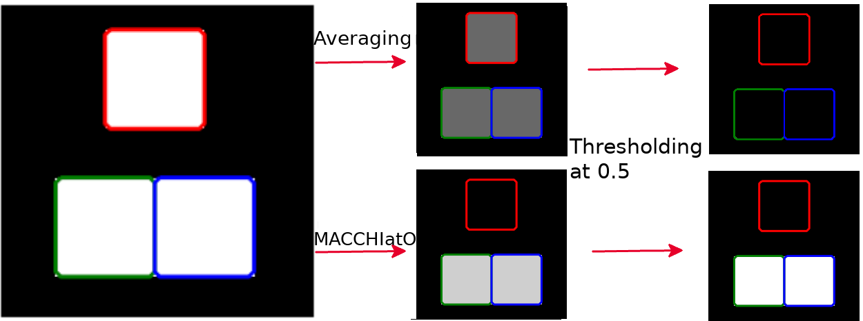
In the remainder, we consider the problem of generating a consensus segmentation , given binary segmentations , of size provided by each rater . The consensus segmentation may be either a hard binary segmentation or a soft probabilistic segmentation , the tilde sign indicating that we are dealing with a continuous probabilistic consensus value, rather than a binary one. Given a soft consensus, one can easily generate a hard consensus by thresholding the soft consensus voxels at the 0.5 limit. Yet, this raises the issue of dealing with voxels that are exactly at the 0.5 value which can be either set arbitrarily to one of the 2 classes or set aside to a third class.
In terms of probabilistic framework, the main approach is to consider that each observed binary segmentation results from a random process applied on a consensus segmentation which is captured by the likelihood distribution also involving some parameters specific to each rater . A prior probability on the consensus is also defined related to the general a priori knowledge about the consensus segmentation. Then a hard consensus can be obtained as a maximum likelihood or maximum a posteriori estimate whereas a soft consensus is obtained as the posterior probability . The parameters are also estimated by maximum likelihood for hard consensuses or maximum marginal likelihood for soft ones.
We make use of the following notations : , , , and are respectively the number of false positives, true positives, false negatives, and true negatives between observed mask and consensus , i.e. .
We consider as baseline methods to create a hard consensus the majority voting (MV) and the ML STAPLE (Maximum Likelihood STAPLE, a binary version of STAPLE) algorithms whereas mask averaging (MA) and STAPLE algorithm are baseline approaches for the soft consensus estimation. We describe below the hypotheses in terms of probability distribution associated with those baseline models and discuss their limitations.
2.1 Majority Voting and Mask Averaging Models
We first make the hypothesis of voxel independence, i.e. that the binary value of each voxel of an observed segmentation mask is independent of the values of other voxels : . Furthermore, we consider that the prior and likelihood probability are simple Bernoulli distributions of the same parameter : . This means that the probability parameter is potentially different for all voxels, but the same for all raters : . Also, the observed masks do not directly depend on the consensus but share the same distribution.
Therefore the likelihood of observing the whole segmentation data is then
where (resp. ) is the number of times voxel is equal to (resp. ) in the observed segmentation masks ,. After maximizing the likelihood, one trivially gets the Bernoulli parameter as , leading to the Mask Averaging consensus formula where the probability of having a foreground voxel is the frequency of positive voxels in the observed masks . To estimate the hard consensus, one needs to maximize thus leading to majority voting : if and if .
Limitations
Majority voting and mask averaging are simple and easy-to-understand mechanisms to choose a consensus. Yet they suffer from the fact that this decision is purely local without any influence from the neighboring pixels. This can lead to situations where the hard consensus includes some isolated voxels or has very irregular boundaries. This is especially true for mask averaging, which does not have any mechanisms to enforce inter-rater consistency and that relies on the implicit assumption that the neighboring voxels of a segmented voxel are likely to be segmented, which is not the case on the boundaries. Another limitation of majority voting is the case where the number of raters is even and therefore many decisions are ambiguous with as many foreground than background voxels. Finally, those simple models assume that all raters’ contributions to the consensus are equal which may not be the case. In particular, an underperforming rater will bias the soft consensus with mask averaging.
2.2 STAPLE model
In the STAPLE algorithm (Warfield et al., 2004), all voxels are also assumed independent but the probability that is equal to depends on whether is a background or foreground voxel, and on the rater . More precisely, and where is the sensitivity of rater and its specificity.
Prior Consensus
The consensus prior probability is here supposed to factorize as the product of voxel priors values . The original STAPLE paper (Warfield et al., 2004) also introduced an Ising Markov random field model as a prior consensus probability to enforce that a voxel prior value depends on that of its neighbors. However, this approach leads to solving iteratively graph cuts problems and is not available in most widely used STAPLE implementations. Instead, the original paper assumes simple independent priors that lead to closed-form updates. Choosing is a non-informative prior but another common choice is to have a spatially uniform value which is the average relative size of the foreground object in the observed segmentation masks. We further consider more general priors of the form , with a constant independent of the image size, and an exponent. The non-informative case corresponds to while the average object size to .
Maximum likelihood STAPLE (ML STAPLE)
The likelihood of the observed data simply writes as and does not involve the prior on the consensus. There is no closed-form expression for the estimation of the rater parameters () and the hard consensus () maximizing the likelihood. But an iterative maximization of the likelihood is possible by setting its derivatives to zero which leads to the update equation :
| (1) | ||||
| (2) | ||||
Maximum marginal likelihood (MML STAPLE)
The marginal likelihood or evidence writes as and is only a function of the rater parameters . Its maximization is not tractable in closed form but the expectation-maximization algorithm provides a way to estimate some local maxima. The E-step consists in evaluating the posterior probability from Bayes law with the current estimated sensitivities and specificities :
| (3) |
.
The M-step updates the parameters and as follows :
| (4) |
where , , , are the ”soft extension” of the number of true positive, true negative, false positive, and false negative voxels from rater .
2.2.1 Influence of the prior term
We can better understand the influence of the prior when estimating the probability to belong to a consensus by writing its logit from Eq.3 :
| (5) |
Thus, we see that to estimate each foreground voxel of rater ”votes” with a (usually) positive quantity whereas each background voxel ”votes” with a (usually) negative quantity . Then the prior term biases this vote depending on whether is greater or smaller than .
2.2.2 Influence of the background size
In many cases, the size of images that contain the objects delineated by the raters is arbitrary since it can be the size of the original image (with a large value of ) or the size of a restricted region of interest (with a small value of ). It is therefore important to estimate the influence of the background size, i.e. the number of true negative voxels , in the estimation of the hard and soft consensus.
Influence on hard consensus
Based on Eqs.1 and 2, the sensitivity and coefficient are not influenced by , but the specificities are. More precisely, we have , and therefore the quantity tends towards when reaches large values. This implies that the hard consensus converges towards the union of all observed segmentation masks when the background size becomes large.
Influence on soft consensus
The posterior probability and specificities are mainly impacted by the increase of the background size, while the sensitivities are more marginally influenced. The nature of the soft consensus depends on the exponent of the prior expression , and in particular we have :
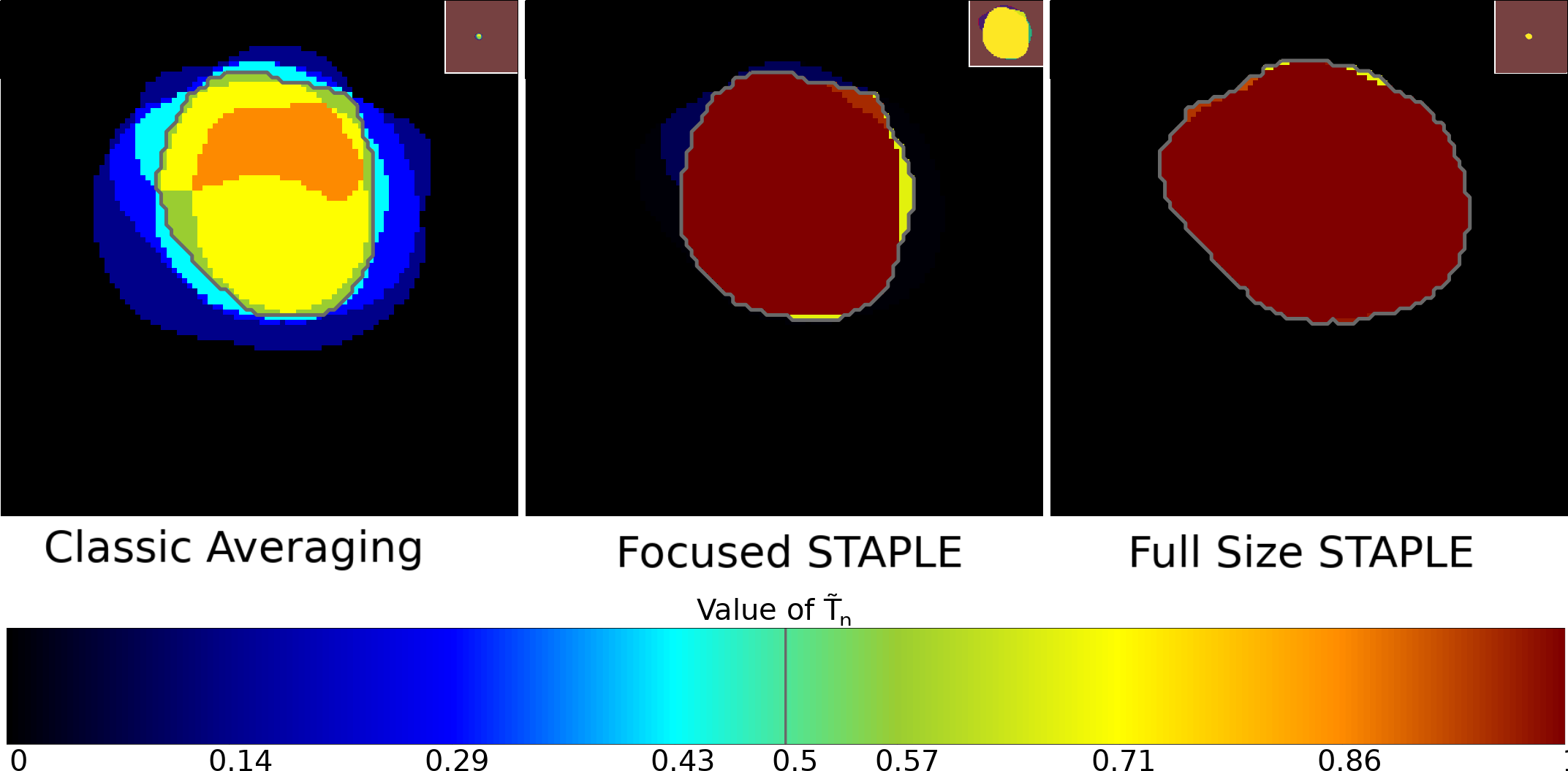
A direct consequence of this formula is that the background size impacts the obtained consensus, as can be seen in Fig. 1(a) where the consensus obtained when applying STAPLE on a bounding box tightly surrounding the organ (referred to as Focused STAPLE in Fig. 1(a)) appears as smaller and with more non-binary values than the one computed on the whole image (referred to as Full size STAPLE in Fig. 1(a)). Comparisons between STAPLE computed on both volumes are available in Tab. 10 in the appendices. Moreover, as seen in Fig.1(b), the soft consensus when having a large background size depends on the value of , with larger corresponding to smaller consensuses. The detailed proof is presented in Appendix A.
Removing the Influence of the background size
We explore under which conditions the STAPLE model leads to consensus estimations that are independent of the background size. A first simplification of the model is to assume that all raters perform equally , . In this case, the global specificity maximizing the likelihood is which is still dependent on the size of the background through .
A second simplification is to consider that each rater sensitivity and specificity are equal, i.e. . This implies that the rater performance is independent of the fact the consensus voxel is in the background or foreground. In this case, the parameter can be interpreted as the accuracy parameter and its optimization leads to . It is easy to see that in that case, , and therefore the maximum likelihood is equivalent to majority voting when which is independent of background size. With this simplification, and from Eq.5, the soft consensus obtained by maximizing the marginal likelihood with a non-informative prior , is such that . The value of depends on the background size, but whether a voxel is more likely to be a background pixel does not depend on the background size.
2.2.3 Limitations
The STAPLE algorithm addresses the problem of taking into account the performance of raters when building a consensus segmentation. However, this approach has the drawback of being dependent on the choice of the prior, and the background size. This dependence of the STAPLE consensus can be explained by the fact that it is a generative model which should explain the foreground and the background voxels separately. When assuming that the rater performance is the same in both background and foreground, then the model becomes equivalent to majority voting. This dependence is a subject of concern as STAPLE is often used as a standard in label fusion works. To improve the robustness of comparisons with novel methods and decrease the impact of this hidden hyperparameter, researchers may compute STAPLE consensus using several bounding boxes, or at least indicates the size of the bounding box on which STAPLE was applied.
The use of local sliding windows in STAPLE as in Commowick et al. (2012) can somewhat mitigate the background size effect, but smaller structures in images can still be impacted and the window size remains a hyperparameter which is difficult to set.
3 MACCHIatO framework
3.1 Main approach description
In the previous section, we have seen that only the majority voting and mask averaging algorithms lead to a consensus that is independent of the background size. Yet, those algorithms are purely local at the voxel level and can lead to irregular boundaries or isolated voxels.
In this section we introduce a new framework to compute soft and hard consensuses that are i) invariant from the background size and ii) dependent on the global morphology of each binary object. This approach is coined MACCHIatO for Morphologically-Aware Consensus Computation via Heuristics-based IterATive Optimization.
Distance-based approach
We formulate the estimation of a hard consensus as the minimization of the sum of the square distance between the consensus and each observed binary mask :
| (6) |
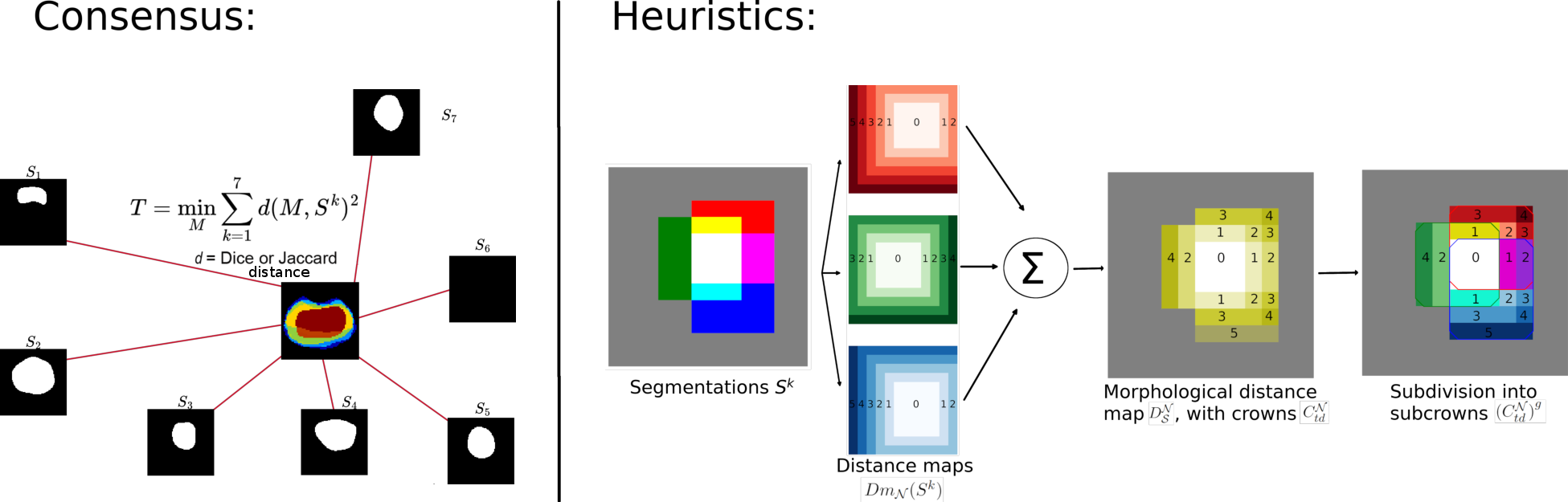
where is a distance as defined in Deza and Deza (2016) between the two masks and . This is equivalent to estimating the consensus as a maximum likelihood where the likelihood can be written as . We can note that the squared sum also corresponds to the definition of a Fréchet variance. Based on this interpretation, appears as the Fréchet mean of i.e. its centroid in the metric space defined by .
Link with baseline models
In section 2.2.2, we have seen that when the sensitivity and specificity are equal, the maximization of the STAPLE model leads to the majority voting algorithm. In this case, we can write the likelihood (where is the accuracy parameter) which is a product of independent Bernoulli distributions. Since the Bernoulli distribution is a member of the exponential family (Dai et al., 2013), it can be also written as where . The number of false positives or false negatives is the number of elements of symmetric difference between the two sets and : and is also called the Hamming distance in information theory. Thus, by choosing , the maximum likelihood leads to majority voting consensus (as detailed in Appendix B).
Soft consensus framework
On the baseline models, soft consensuses were obtained as posterior probabilities of having a consensus from the observed binary masks. However, from the likelihoods , the computation of the posterior may not be tractable due to the difficulty of computing the normalization constant. Instead, we propose to approximate by the quantity such that minimizes the quantity :
| (7) |
where is a distance between the probabilistic array and the binary mask . More precisely, the distances considered are soft surrogate of the distance between binary sets such that when . For instance, the distance is a soft surrogate of the Hamming distance since . Besides it is clear that the mask averaging (MA) method is a soft consensus minimizing the following squared sum .
Optimization approach
The estimation of the soft and hard consensus is independent of the background size if the distance is invariant to the number of true negatives. Besides, unlike the MV and MA algorithms, the optimization cannot be performed at the voxel level when the distance cannot be split voxelwise. Instead of optimizing the whole foreground object, we chose to consider each connected component separately from each other to obtain more coherent results. Finally, we further split the optimization into subcrowns with various heuristics to speed up the computation.
3.2 Distances between binary masks
We detail below the selected distances between binary sets that are considered and their associated soft surrogates. We mainly focus on distances based on two widely used methods to measure the overlap between binary segmentations : the Jaccard and Dice coefficients.
Jaccard distance
The Jaccard coefficient (aka IoU) between binary masks and is defined as : . In Kosub (2019), it is shown that its complementary to 1 is a metric between binary sets following the triangular inequality. Several formulations of soft surrogates exist that extend the Jaccard distance. We focused specifically on two of them : the Soergel metric (Späth, 1981; Deza and Deza, 2016) which follows the triangular inequality but is not differentiable, and the widely-used Tanimoto distance (Willett et al., 1998; Deza and Deza, 2016; Leach and Gillet, 2007) .
Dice coefficient
It is defined as and is widely used in image segmentation as a performance index. Indeed, the Dice index is equal to the F1-score and corresponds to the harmonic mean of the sensitivity and positive predictive value. It is closely related to the Jaccard coefficient as . The Dice distance is a near-metric i.e. it respects a relaxed form of the triangular inequality (Gragera and Suppakitpaisarn, 2018). Soft surrogates of the Dice distance have been developed especially as a loss function in deep learning. We consider in the remainder two main extensions of the Dice distance (Ma et al., 2021) on non-binary sets defined as where .
By construction, all those distances only depend on segmented pixels and are independent of the background size. Note that both distances are extended to get a null distance between two empty sets. Using those distances in the Fréchet variance computation, the inclusion of voxels segmented by a large number of raters (resp. a few raters) decreases (resp. increases) its value. The different formulations of the MACCHIatO framework are summarized in table 1.
| Hard ConsensusMethod | Soft ConsensusMethod | Distance | Soft Surrogate | Computation-level |
|---|---|---|---|---|
| Majority Voting | Mask Averaging | Voxel-level | ||
| ML STAPLE | MML STAPLE | NA | NA | Image-level |
| MACCHIatO-J | MACCHIatO-TJ | Jaccard | Tanimoto | Connectedcomponentlevel |
| MACCHIatO-SJ | Soergel | |||
| MACCHIatO-D | MACCHIatO-1SD | Dice | ||
| MACCHIatO-2SD |
3.3 Heuristic computation based on morphological distance and crowns
Domain of optimization
Since the distances listed in the previous section are independent of the number of true negatives, their computations can be restricted to the union of all rater masks : . Furthermore, we consider that to decide whether a voxel belongs to the consensus, one should only take into account the regional context associated with the connected components surrounding that voxel, since far-away components may not be relevant. Therefore, we choose to minimize separately the Fréchet variances of Eqs. 6 and 7 for each connected component of the masks union . Therefore, in practice, we minimize the Local Mean Squared Distance between and the consensus : where (resp. ) are the restriction of the binary masks (resp. ) to the connected component . A benefit of this choice is that the determination of the Fréchet Mean behaves similarly to a structure-wise MV, as the Fréchet Mean of components segmented by less than half of the raters is the null set. However, contrary to MV, raters who do not segment a component kept by the majority of raters do not bias its consensus segmentation, as their contribution to the associated LMSD is = 0 and does not impact the Fréchet mean. To lighten notations, we drop the index in the remainder. It is equivalent to considering that has only one single connected component.
Subcrown-based optimization
The minimization of the Fréchet variance is a combinatorial problem with a complexity of for the naive approach. Furthermore, it may lead to several global minima when the number of raters is small. For those reasons, we propose instead to seek a local minimum of the Fréchet variance by introducing some heuristics in the optimization. With this approach, the local minimum has a lower complexity to compute and, by construction, is maximally connected to avoid isolated voxels.
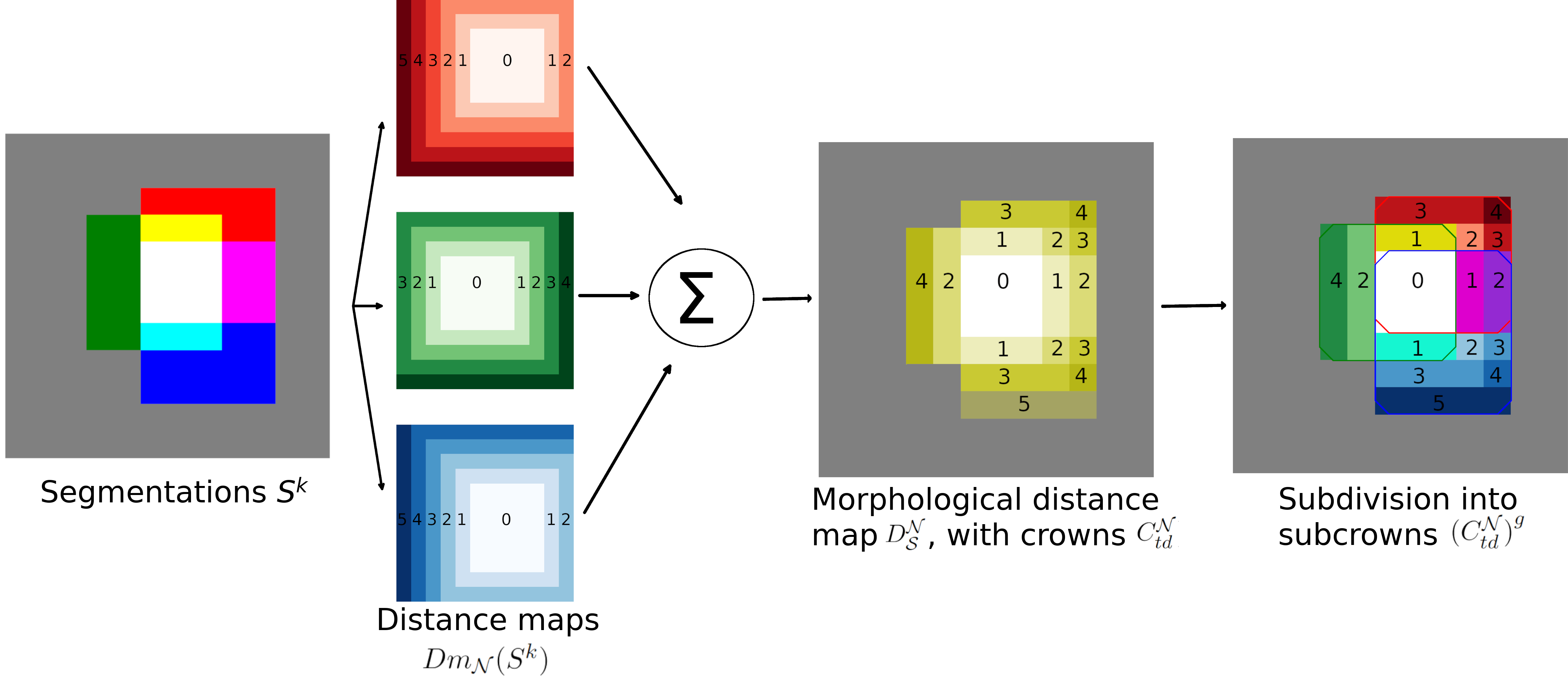
More precisely, instead of a computationally expensive per voxel minimization of the Fréchet variance, we decompose the set into a set of subcrowns that take into account the global morphological relationships between each rater mask. The formal definition of subcrowns requires the specification of distance maps to each binary mask on according to a chosen neighborhood . This one can be either the 4 or 8 (resp. 6 or 26) connectivity in 2D (resp. 3D). The distance is set to 0 for all voxels inside the object .
The global morphological distance map is the sum of those distance maps
for all raters on . A crown is defined as the set of voxels having the same global morphological distance . Those crowns realize a partition of (), and the -crown corresponds by construction to the intersection of all masks in .
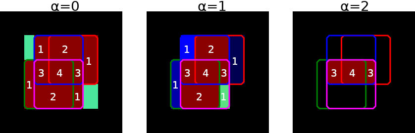
We further split each crown as a set of subcrowns by grouping the voxels that have been produced by the same set of raters. In other words, a subcrown corresponds to a set of voxels located at the same morphological distance from the intersection of all rater masks and which have been segmented by the same group of raters, as seen in Fig. 2(a). Formally, a subcrown is noted where the superscript corresponds to a group of raters and subcrowns realize a partition of a crown :
| (8) |
where is the power set (i.e. the set of all subsets) of the first K integers.
The process for the construction of subcrowns is illustrated in Fig. 2(a)
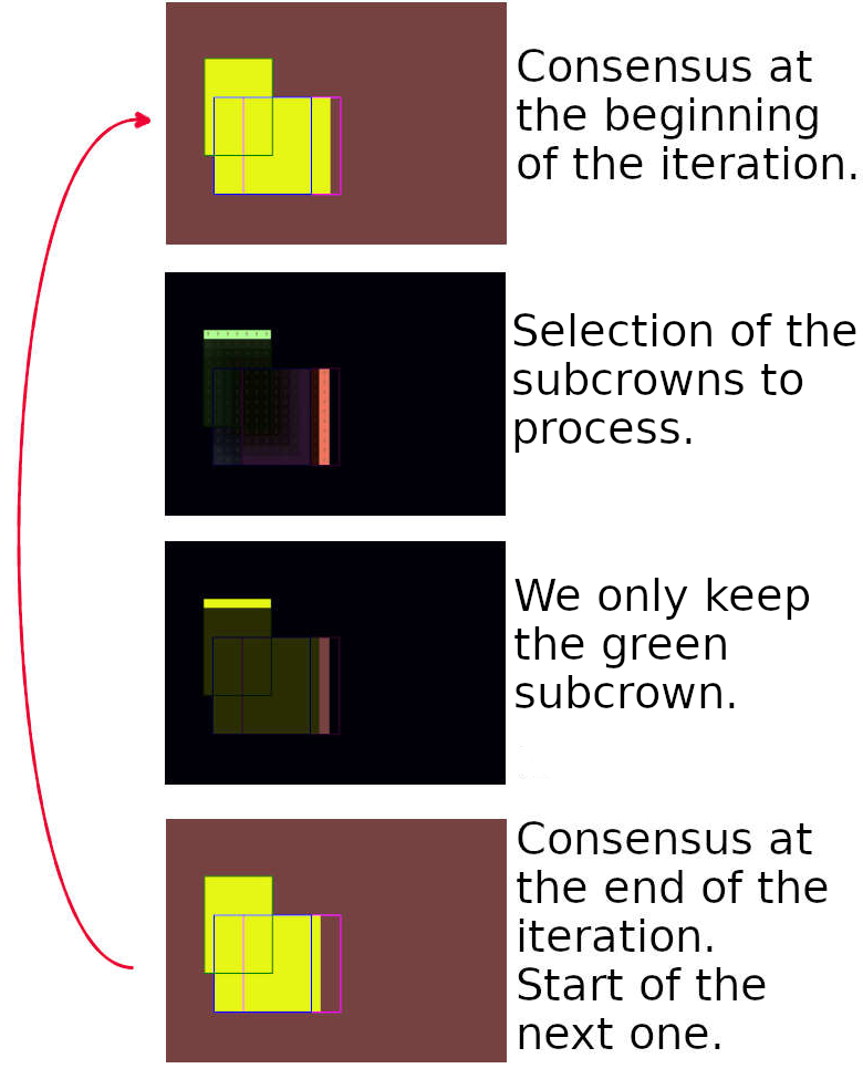
3.4 Hard consensus algorithm
The optimization proceeds in a greedy fashion by iteratively removing or adding subcrowns to the current estimate of the consensus until the criterion stops decreasing. In Alg. 1, we use two concurrent strategies : either we start from the union of all masks and then remove subcrowns with decreasing distances (a straegy illustrated in Fig. 2(b), or we start with the crown with the minimum distance and then add subcrowns of increasing distances. Both growing and shrinking strategies are applied as the greedy process can lead to different results, and we keep the consensus associated with the minimum of both strategies and the null set. The latter is also tested in the last stage since the distance of a set to the null set is , for both Dice and Jaccard distances. This discontinuity is not compatible with the iterative process and calls for a independent test.
Examples of consensuses obtained with this strategy can be seen in Fig. 3. Thus, the resulting consensus leads to a consistent grouping since all voxels belonging to the same connected component, having the same morphological distance, and being generated by the same group of raters will end up in the same class. Alternative optimization approaches could have been based on adding or removing single voxels (smaller than subcrowns) or crowns (larger than subcrowns). While voxel-based minimization would be very time-consuming, especially in 3D, conversely crown-based would lead to suboptimal results as crowns can be fairly large. Thus, the Morphologically-Aware Consensus Computation via Heuristics-based IterATive Optimization (MACCHIatO) algorithm is designed to be a good compromise between computational efficiency and consistency, with a number of iterations exponentially depending on but which is lower than the naive complexity.
3.5 Soft consensus algorithm
The estimation of a probabilistic or soft consensus is based on the minimization of the sum of square surrogate distances as displayed in Eq. 7 and the optimization is split for each connected component of the mask union .
The soft MACCHIatO algorithm extends the previous approach to minimize the criterion . A brute force approach would lead to the optimization of a sum of rational polynomials over a set of scalars. Instead, we proceed in a greedy manner, separately on each connected component of , by starting with the mean consensus and optimizing successively subcrowns of increasing distances. All subcrowns of increasing distances are iteratively considered until stops decreasing. For each subcrown , we seek the scalar value such that it minimizes
The algorithm is described in Alg.2 and iteratively optimizes each subcrown from the inside to the outside of the set. We have observed no gain in combining a growing and a shrinking exploration of subcrowns contrary to Alg. 1. For the optimization process of Eq. 3.5, we use the SLSQP algorithm (Kraft, 1988) implemented in Scipy v1.7.3 (Virtanen et al., 2020). Resulting consensus can be seen in Figs. 4, 6 and 7.
4 Results
4.1 Datasets and Implementation Details
We tested our method on 3 datasets :
- •
A private database of transition zones of prostate T2w MR images, composed of 40 cases segmented by 5 raters.
- •
The publicly available MICCAI MSSEG 2016 dataset of Multiple Sclerosis lesions segmentations (Commowick et al., 2018) segmented from Brain MR images, with 15 subjects segmented by 7 raters
- •
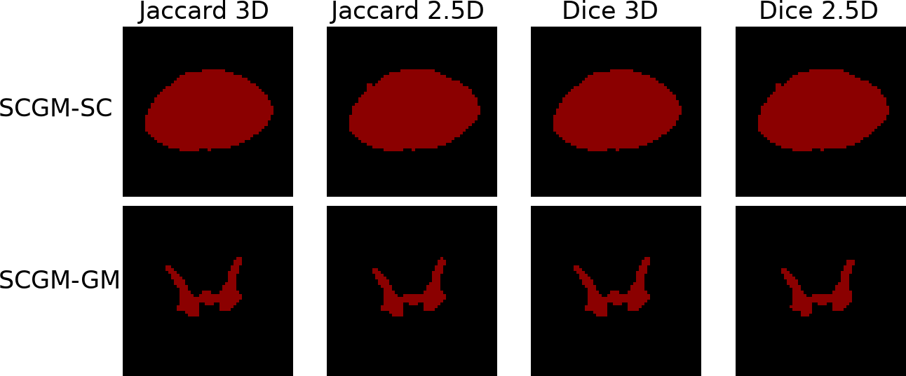
The publicly available SCGM dataset (Prados et al., 2017), with 40 spinal cords and their grey matter segmented by 4 raters. We used the whole spinal cord segmentation (SCGM-SC) and the grey matter segmentation (SCGM-GM).
Images from the private dataset (resp. MSSEG dataset, SCGM dataset) have a size of [80-288][320-640][320-640] voxels (resp. [144-261][224-512][224-512] voxels and [3-28][100-655][100-776] voxels). It was possible to extract from the private dataset bounding boxes of size [58-227][53-184][62-180] voxels. Similarly, we were able to extract from SCGM-SC (resp. SCGM-GM) bounding boxes of size [3-20][15-90][24-131] voxels(resp.) From the 3D private dataset, we created a 2D subset by extracting a single slice for each patient located at the base of the prostate since this region is subject to a high inter-rater variability (Becker et al., 2019; Montagne et al., 2021).
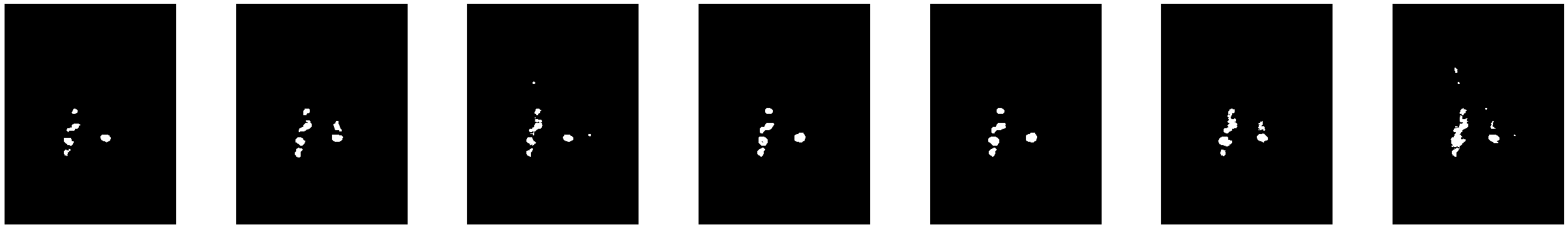
Examples for each dataset of segmentations by the different raters of the same case are available in Appendix C (Fig. 8).
Implementation details
In the remainder, STAPLE results were produced by using the algorithm implemented in SimpleITK v2.0.2 (Lowekamp et al., 2013). All MACCHIatO methods used the 8 or 26-connectivity neighborhood for 2D or 3D cases. MACCHIatO code is available at https ://gitlab.inria.fr/dhamzaou/jaccardmap
4.2 Heuristics relevance
In Section 3.3, we have presented the subcrown-based heuristics that drives the optimization of the local mean square distance criteria. Indeed, those subcrown group voxels are based on three properties : their morphological distance, the connected component they belong to, and the raters who segmented them. To check if this heuristics is appropriate, we compared it with two alternatives :
- •
- •
The other one iteratively processes each voxel separately.
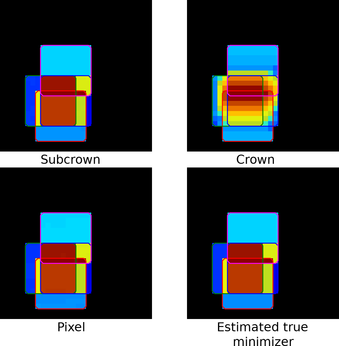
We compared the 3 heuristics by computing a soft consensus (with the Tanimoto distance) on the toy example of Fig. 5, and we display their optimized value of and their computation time in Table 2. Furthermore, since the size of is small, we could estimate the true minimizer of that involves the optimization of parameters.
Unlike the crown-based heuristics, the subcrown-based and voxel-based heuristics appear to compute a consensus close to the real minimizer. In addition, the subcrown method is significantly faster than the voxel-based approach.
We have also compared the three heuristics on two datasets in Table 3. The crown-based heuristics is the fastest method to compute but with the highest criteria , whereas the voxel-based method requires far more computation time than the subcrown-based heuristics and even several hours for some Prostate 3D cases. Surprisingly, on average, the subcrown-based heuristics reaches a lower criteria than the voxel-based method, although the difference may hardly be seen in the produced consensus. On those datasets, we were not able to estimate the true minimizer of , due to the high memory resources those computations would require.
| Heuristics | Time | |
|---|---|---|
| Subcrown-basedheuristics | 0.159 | 0.26s |
| Crown-basedheuristics | 0.176 | 0.07s |
| Voxel-basedapproach | 0.159 | 0.92s |
| Estimated Trueminimizer | 0.159 | 0.55s |
| Dataset | Subcrown | Crown | Voxel |
|---|---|---|---|
| MSSEG | 16.36 (57.48s) | 16.50 (23.41s) | 16.36 (20min30s) |
| Prostate 3D | 1.24e-2 (31.5s) | 1.26e-2 (5.46s) | NA |
| Prostate 2D | 5.98e-3 (0.29s) | 6.22e-3 (0.07s) | 6.10e-3 (5.30s) |
4.3 Comparison with baseline methods
Comparison of inter-rater variabilities
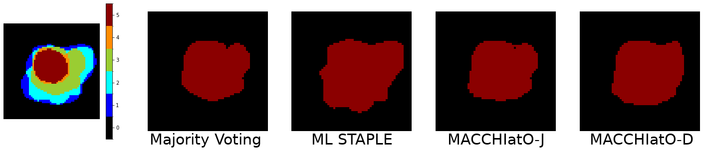
A first set of experiments consist in measuring the impact of the choice of the consensus method when computing a measure of inter-rater variability. More precisely, we compute the average precision, recall, and F1-score between the hard consensus (considered as ground truth) and each rater segmentation. Those metrics have been computed on the MSSEG dataset where there are potentially large disagreements between raters. Table 4 reports those metrics averaged among all lesions of all images, a lesion corresponding to a connected component of the mask union . The MV consensus has the highest recall and lowest precision which can be interpreted by a MV consensus smaller than other methods. Conversely, the STAPLE consensus has the largest precision and lowest recall, thus corresponding to a larger size consensus. Regarding terms of F1-score, MV and MACCIHIatO methods obtained similar metrics but slightly higher for MACCHIatO-D (0.449).
| MLSTAPLE | MV | MACCHIatO-J | MACCHIatO-D | |
|---|---|---|---|---|
| Precision | 0.976 | 0.497 | 0.562 | 0.570 |
| Recall | 0.273 | 0.817 | 0.769 | 0.758 |
| F1-score | 0.297 | 0.437 | 0.448 | 0.449 |
In addition, we also compared the methods on the number of connected components. To do so, we defined each consensus as ground truth and from there computed the average precision, recall, and F1-score of each rater for lesion detection (considering the existence of a non-null intersection with the rater’s segmentation as a sufficient threshold to detect). We performed this experiment on the MSSEG dataset, as it is our only dataset with several connected components per case. Table 5 reports those metrics averaged among all patients. The MV consensus has the highest detection recall and lowest detection precision which can be interpreted by a MV consensus not segmenting some lesions conserved by the other methods. Conversely, the STAPLE consensus has the largest precision and lowest recall, thus corresponding to the presence of lesions rarely segmented by the raters. In terms of F1-score, MV and MACCHIatO methods are close to each other, but it is highest for MACCHIatO-D (0.894).
| MLSTAPLE | MV | MACCHIatO-J | MACCHIatO-D | |
|---|---|---|---|---|
| Precision | 0.994 | 0.887 | 0.914 | 0.931 |
| Recall | 0.643 | 0.967 | 0.931 | 0.930 |
| F1-score | 0.746 | 0.892 | 0.888 | 0.894 |
Comparison of consensus areas or volumes
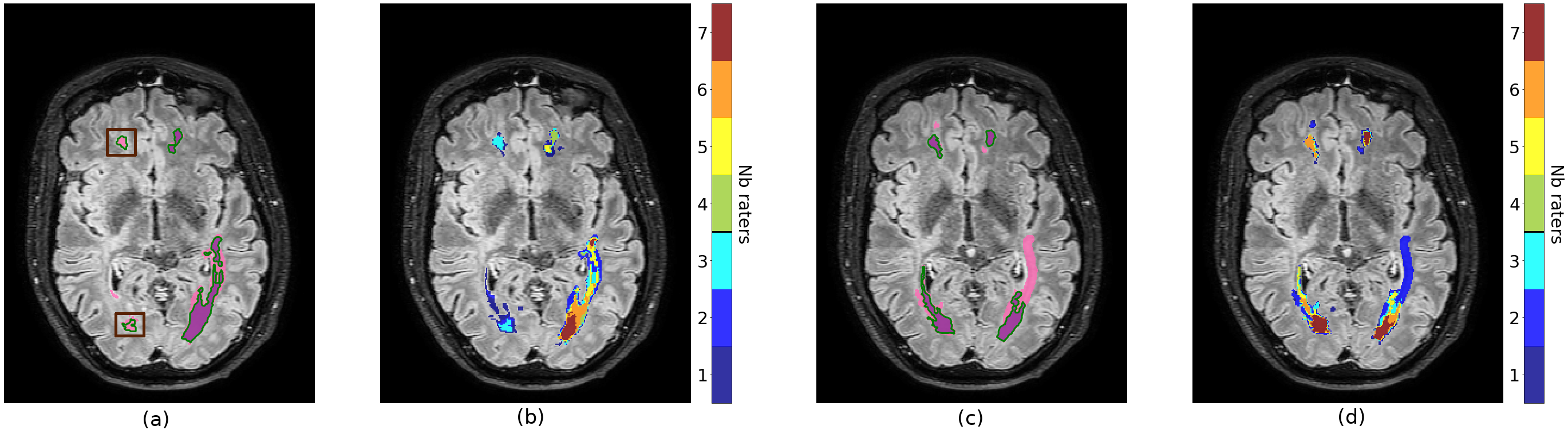
In Table 6, we compare the relative size of hard consensuses on all datasets, taking the MV consensus as reference. On average, all methods lead to consensuses of larger size than MV. For the MACCHIatO methods, the difference with MV consensus is modest on a massive organ (prostate) but significant for small lesions (16%). The ML STAPLE method generates much larger consensuses than MV, especially when dealing with small lesions. Note that for the MSSEG dataset, ML STAPLE is computed on the whole image, thus with a large background size. Finally, the MACCHIatO-D and MACCHIatO-J methods lead to consensuses of similar size, without any clear order. Table 7 compares the soft area or volumes of the soft consensuses (given by ) generated by all methods, taking the mask averaging as reference. Fig. 6 illustrates those soft consensuses on the MSSEG dataset. The variation of volumes is smaller for soft consensus than for hard consensus. In general, the MA method produces the smallest volumes, and STAPLE the largest ones. The methods using surrogate Dice or Jaccard distances give similar volumes, although the Soergel and are more diverging on the MSSEG dataset. We also compare the size of the thresholded maps which provide similar trends to their soft maps.
For both hard and soft consensuses, the largest differences between the different methods are observed on the MSSEG dataset, followed by SCGM-GM.
| Avg. size variation w.r.t MV | Frequencies of size | |||||
|---|---|---|---|---|---|---|
| Jaccard | Dice | ML STAPLE | Jaccard | Dice | ML STAPLE | |
| Prostate 3D | +0.4% | +0.6 % | +22% | 87.5% | 85% | 100% |
| MSSEG | +19% | +16% | +151% | 100% | 93% | 100% |
| SCGM-SC | +2.36% | +2.30% | +11% | 97.5% | 97.5% | 100% |
| SCGM-GM | +17% | +15% | +47% | 100% | 100% | 100% |
| Avg. soft volume variation w.r.t MA | |||||
| TJ | SJ | 2SD | 1SD | STAPLE | |
| Prostate 3D | +0.4% | +0.1% | +0.1% | +0.7% | +10% |
| Thresholded | +0.1% | +0.07% | +0.09% | +0.03% | +11% |
| MSSEG | +4% | +16% | +2% | -3% | +43% |
| Thresholded | +8% | +37% | +4% | +11% | +68% |
| SCGM-SC | -0.4% | +0.5% | -0.5% | +0.3% | +4% |
| Thresholded | +1% | +1.3% | +0.9% | +0.9% | +5.7% |
| SCGM-GM | +1.2% | +4.4% | +1% | +2.9% | +8.6% |
| Thresholded | +13% | +16% | +11% | +14% | +19% |
| Frequencies of soft volume | ||||
| TJ | SJ | 2SD | 1SD | |
| Prostate 3D | 80% | 65% | 60% | 80% |
| Thresholded | 22.5% | 12.5% | 7.5% | 7.5% |
| MSSEG | 87% | 100% | 73% | 33% |
| Thresholded | 93% | 100% | 80% | 93% |
| SCGM-SC | 10% | 52.5% | 5% | 37.5% |
| Thresholded | 35% | 67.5% | 25% | 27.5% |
| SCGM-GM | 92.5% | 95% | 92.5% | 82.5% |
| Thresholded | 100% | 100% | 100% | 100% |
We recorded the cumulative running time for STAPLE and soft MACCHIatO methods to generate a consensus for all structures of our datasets in Table 8. We did not consider MA as it requires far less computation than the other methods. Among the considered algorithms STAPLE is in general the fastest method, being approximately 2-3 times faster than MACCHIatO methods. The exception here is the computation time on SCGM, which always involves small structure sizes and large image sizes.
| TJ | SJ | 2SD | 1SD | STAPLE | |
| Prostate 2D | 11.1s | 14.6s | 7.4s | 9.8s | 2.3s |
| Prostate 3D | 15m02s | 12m52s | 9m19s | 9m48s | 4m17s |
| MSSEG | 14m29s | 11m31s | 11m42s | 11m13s | 3m38s |
| SCGM-SC | 16.7s | 15.1s | 14s | 14.3 | 40.6s |
| SCGM-GM | 14.1s | 12.8s | 12.4s | 13.3s | 34.7s |
4.4 Entropy of soft consensus
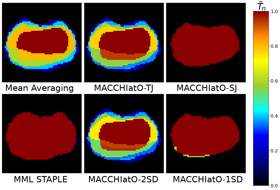
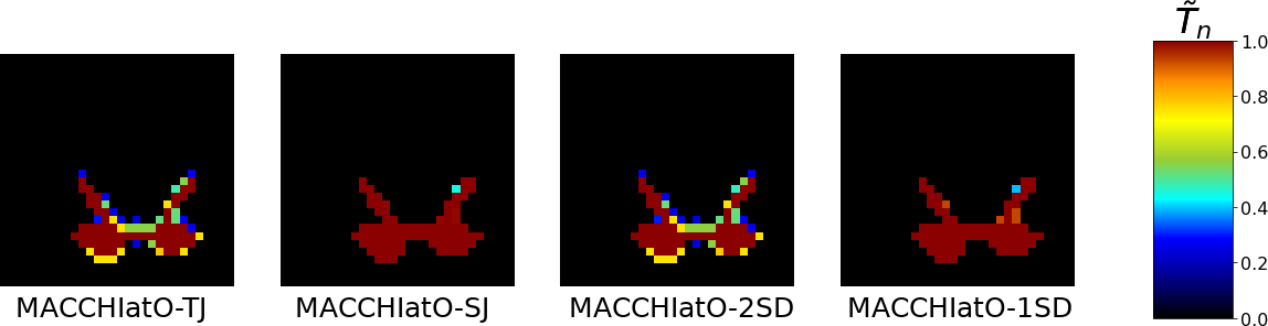
In Figs. 3 and 7 we show examples of soft consensuses on the prostate and grey matter datasets. It appears that MACCHIatO-SJ and MACCHIatO-1SD methods often assign to subcrowns probability values very close to 0 or 1 despite being soft consensus methods. To confirm this behaviour, we compared on all 3D datasets the Shannon entropy obtained by MA and by the four soft MACCHIatO methods. Table 9 confirms the strong binary behavior of MACCHIatO-SJ and MACCHIatO-1SD methods while MACCHIatO-TJ and MACCHIatO-2SD have a similar spread than mask averaging. Thus, we classify the surrogate distances between two families : the ones associated with low-entropy consensus (Soergel, ), and the ones generating high-entropy consensus (Tanimoto, ).
| Dataset | MA | TJ | SJ | 2SD | 1SD |
|---|---|---|---|---|---|
| Prostate 3D | 63850 | 63658 | 6928 | 63799 | 19361 |
| MSSEG | 41295 | 37377 | 3805 | 37720 | 6107 |
| SCGM-SC | 2401 | 2467 | 259 | 2483 | 305 |
| SCGM-GM | 757 | 736 | 97 | 736 | 118 |
4.5 Discussion
Experiments confirmed the dependence on background size of the STAPLE method, as shown in Fig. 1(a) and Appendix A (Tab. 10). We also observed that hard consensuses obtained by MACCHIatO were generally slightly larger than those obtained by MV, particularly with MACCHIatO-J which almost never produces consensuses smaller than MV’s. This can be explained by the fact that the MACCHIatO consensus may include voxels segmented by less than half of the raters (as seen in Figs. 3 and 6). Finally, STAPLE consensuses always have a larger size than both MACCHIatO and MV. Similar observations can be made on soft consensus but with a smaller difference between methods on soft volumes compared to hard volumes. The MACCHIatO methods by construction create consensuses, independent from the background size, that maximize the local average (soft) squared Dice or Jaccard coefficients between the consensus and rater masks for each connected component. Furthermore, they produce masks that are different from the MV and STAPLE methods and have in general larger volumes than MV consensuses and smaller volumes than STAPLE ones. Finally, the MACCHIatO algorithms are in general more computationally expensive than MV or STAPLE algorithms but only to a reasonable extent (about 2 or 3 times more). In this article, we had the deliberate position not to choose between soft and hard consensus. From our perspective, the choice of method should be based on the users’ motivations and the downstream task. If the users solely aim to generate a binary mask for visualization purposes or inter-rater variability studies, they can opt for the hard consensus method. However, if they wish to incorporate uncertainty modeling and obtain more refined results, the soft consensus methods would be more suitable.
Similarly, the choice of distances should align with the intended objectives. If users prioritize a solid mathematical foundation for the method, then they may opt for the Jaccard (hard) and Soergel (soft) metrics as, contrary to other used distances, they respect the triangular inequality. Alternatively, the Tanimoto distance can be used for uncertainty assessment, as MACCHIatO-TJ outputs more non-binary values than MACCHIatO-SJ. Users also have the flexibility to use the more commonly employed Dice instead of Jaccard if they prefer. In definitive, we have presented a range of methods within a consistent framework and elaborated on their characteristics. However, the specific configuration is ultimately left to the users based on their individual requirements and preferences.
It can also be noted that the size variation observed on a dataset seems to be correlated with its inter-rater variability, the observed differences being more important on the MSSEG and SCGM-GM dataset than on the others.
In this article, we always considered 8-connexity in 2D cases and 26-connexity in 3D cases, as it performed better in preliminary experiments. However, the use of other neighborhoods (such as the 4-neighborhood in 2D, or the 6 and 18-neighborhood in 3D) could be envisaged. Moreover, we did not consider the case of highly anisotropic images, like in the SCGM dataset where a ratio of anisotropy greater than 10 in the voxel size is encountered. For those cases, it could be considered to apply a 2.5D approach consisting in applying our method to each slice independently. Comparisons between 2.5D and 3D neighborhoods on SCGM are available in Appendix D.
The proposed method has several limitations. First, we only considered a binary segmentation problem. Extension to multiclass segmentation could be foreseen using for instance the generalization method presented in Crum et al. (2006) and Sudre et al. (2017). Second, the considered distances between binary sets are based on region overlap measures (Dice, Jaccard indices) and discard distances between boundaries such as Hausdorff Distance (HD). Our experiments based on HD were not conclusive.
The reasons for this may be similar to the ones described in Karimi and Salcudean (2019) : instability of the methods to minimize a distance only defined from the largest error, HD sensitivity to outliers, difficulties to optimize it from an optimization point of view. To mitigate those effects, we made some tests using two of the Hausdorff alternatives defined in Karimi and Salcudean (2019) and based respectively on distance maps and erosion, to no avail.
Third, the proposed criteria , weights all raters equally for all connected components, unlike the STAPLE algorithm. It is possible to extend the MACCHIatO framework by attributing weights to raters based on their precision and recall (as those measures are independent of background size), either at the local or global level. Yet, this extension would require additional optimization steps, since the weights depend on the current estimate of the consensus.
Extending the MACCHIatO method to generate consensuses from (soft) probability maps instead of binary segmentations is not straightforward. Indeed, while minimizing the Fréchet variance of Eq. 7 is well-posed, we can no longer restrict its computation to the set and define subcrowns as optimization blocks. An alternative method that we have explored in our prior workAudelan et al. (2020), is to map probabilities to real values through a link function (e.g. a logit function) and then use robust parametric models (t-distributions) to fuse the probability maps.
5 Conclusion
In this paper, we have shown that the STAPLE method is impacted by the image background size and the choice of prior law. We have also introduced a new background-size independent method to generate a consensus based on Jaccard and Dice-based distances, thus extending the Majority Voting and mean consensus methods. More precisely, the generated masks minimize the average squared Jaccard or Dice distance between the consensus and each rater segmentation. The MACCHIatO algorithms are efficient and provide consistent masks by taking into account local morphological configurations between rater masks. The consensus masks are usually larger than those generated by the majority voting or mask averaging methods but smaller than those issued by STAPLE. Therefore, based on the experiments performed on three datasets, we believe that the hard and soft MACCHIatO algorithms are good alternatives to MV-based and STAPLE-based methods to define consensus segmentation.
Acknowledgments
This work has been supported by the French government, through the 3IA Côte d’Azur Investments and UCA DS4H Investments in the Future project managed by the National Research Agency (ANR) with the reference numbers ANR-19-P3IA-0002 and ANR-17-EURE-0004 and by the Health Data Center of the AP-HP (Assistance Publique-Hôpitaux de Paris). Private data was extracted from the Clinical Data Warehouse of the Greater Paris University Hospitals (Assistance Publique-Hôpitaux de Paris). We thank Julien Castelneau, software Engineer Inria, for his help in the development of MedInria Software (MedInria - Medical image visualization and processing software by Inria https~://med.inria.fr/ - RRID :SCR_001462). The authors are grateful to the OPAL infrastructure from Université Côte d’Azur for providing resources and support. We also thank Alexandre Allera, Malek Ezziane, Anna Luzurier, Raphaelle Quint and Mehdi Kalai for providing prostate segmentations, Yann Fraboni and Etrit Haxholli for insightful discussions, and Federica Cruciani and Lucia Innocenti for feedback.
This paper is dedicated to the memory of our dear colleague Olivier Commowick who has been very active and innovative in the domain of data fusion.
Ethical Standards
The work follows appropriate ethical standards in conducting research and writing the manuscript, following all applicable laws and regulations regarding treatment of animals or human subjects.
Conflicts of Interest
We declare we do not have conflicts of interest
References
- Aljabar et al. (2009) P. Aljabar, R.A. Heckemann, A. Hammers, J.V. Hajnal, and D. Rueckert. Multi-atlas based segmentation of brain images: Atlas selection and its effect on accuracy. NeuroImage, 46(3):726–738, 2009. ISSN 1053-8119. doi: 10.1016/j.neuroimage.2009.02.018.
- Asman and Landman (2012) Andrew Asman and Bennett Landman. Formulating Spatially Varying Performance in the Statistical Fusion Framework. Medical Imaging, IEEE Transactions on, 31:1326–1336, 06 2012. doi: 10.1109/TMI.2012.2190992.
- Asman and Landman (2013) Andrew J. Asman and Bennett A. Landman. Non-local statistical label fusion for multi-atlas segmentation. Medical Image Analysis, 17(2):194–208, 2013. ISSN 1361-8415. doi: 10.1016/j.media.2012.10.002.
- Audelan et al. (2020) Benoît Audelan, Dimitri Hamzaoui, Sarah Montagne, Raphaële Renard-Penna, and Hervé Delingette. Robust Fusion of Probability Maps. In Anne L. Martel, Purang Abolmaesumi, Danail Stoyanov, Diana Mateus, Maria A. Zuluaga, S. Kevin Zhou, Daniel Racoceanu, and Leo Joskowicz, editors, Medical Image Computing and Computer Assisted Intervention - MICCAI 2020, pages 259–268, Cham, 2020. Springer International Publishing. ISBN 978-3-030-59719-1.
- Becker et al. (2019) Anton S. Becker, Krishna Chaitanya, Khoschy Schawkat, Urs J. Muehlematter, Andreas M. Hötker, Ender Konukoglu, and Olivio F. Donati. Variability of manual segmentation of the prostate in axial t2-weighted mri: A multi-reader study. European Journal of Radiology, 121:108716, 2019. ISSN 0720-048X. doi: https://doi.org/10.1016/j.ejrad.2019.108716.
- Commowick et al. (2012) Olivier Commowick, Alireza Akhondi-Asl, and Simon K. Warfield. Estimating A Reference Standard Segmentation with Spatially Varying Performance Parameters: Local MAP STAPLE. IEEE Transactions on Medical Imaging, 31(8):1593–1606, August 2012. doi: 10.1109/TMI.2012.2197406.
- Commowick et al. (2018) Olivier Commowick, Audrey Istace, Michael Kain, Baptiste Laurent, Florent Leray, Mathieu Simon, Sorina Camarasu Pop, Pascal Girard, Roxana Ameli, Jean-Christophe Ferré, Anne Kerbrat, Thomas Tourdias, Frédéric Cervenansky, Tristan Glatard, Jeremy Beaumont, Senan Doyle, Florence Forbes, Jesse Knight, April Khademi, Amirreza Mahbod, Chunliang Wang, Richard Mckinley, Franca Wagner, John Muschelli, Elizabeth Sweeney, Eloy Roura, Xavier Llado, Michel Santos, Wellington P Santos, Abel G Silva-Filho, Xavier Tomas-Fernandez, Hélène Urien, Isabelle Bloch, Sergi Valverde, Mariano Cabezas, Francisco Javier Vera-Olmos, Norberto Malpica, Charles R G Guttmann, Sandra Vukusic, Gilles Edan, Michel Dojat, Martin Styner, Simon K. Warfield, François Cotton, and Christian Barillot. Objective Evaluation of Multiple Sclerosis Lesion Segmentation using a Data Management and Processing Infrastructure. Scientific Reports, 8(1):13650, December 2018. doi: 10.1038/s41598-018-31911-7.
- Crum et al. (2006) William Crum, Oscar Camara, and Derek Hill. Generalized Overlap Measures for Evaluation and Validation in Medical Image Analysis. IEEE transactions on medical imaging, 25:1451–61, 12 2006. doi: 10.1109/TMI.2006.880587.
- Dai et al. (2013) Bin Dai, Shilin Ding, and Grace Wahba. Multivariate Bernoulli distribution. Bernoulli, 19(4):1465–1483, 2013.
- Dewalle-Vignion et al. (2015) Anne-Sophie Dewalle-Vignion, Nacim Betrouni, Clio Baillet, and Maximilien Vermandel. Is STAPLE algorithm confident to assess segmentation methods in PET imaging? Physics in Medicine and Biology, 11 2015. doi: 10.1088/0031-9155/60/24/9473.
- Deza and Deza (2016) Michel Marie Deza and Elena Deza. Distances and Similarities in Data Analysis. In Encyclopedia of Distances, pages 327–345, Berlin, Heidelberg, 2016. Springer Berlin Heidelberg. ISBN 978-3-662-52844-0. doi: 10.1007/978-3-662-52844-0˙17.
- Gragera and Suppakitpaisarn (2018) Alonso Gragera and Vorapong Suppakitpaisarn. Relaxed triangle inequality ratio of the Sørensen–Dice and Tversky indexes. Theoretical Computer Science, 718:37–45, 2018. ISSN 0304-3975. doi: https://doi.org/10.1016/j.tcs.2017.01.004. URL https://www.sciencedirect.com/science/article/pii/S0304397517300361. WALCOM (Workshop on Algorithms and Computation).
- Hamzaoui et al. (2022) Dimitri Hamzaoui, Sarah Montagne, Raphaële Renard-Penna, Nicholas Ayache, and Hervé Delingette. Morphologically-aware jaccard-based iterative optimization (mojito) for consensus segmentation. In Carole H. Sudre, Christian F. Baumgartner, Adrian Dalca, Chen Qin, Ryutaro Tanno, Koen Van Leemput, and William M. Wells III, editors, Uncertainty for Safe Utilization of Machine Learning in Medical Imaging, pages 3–13, Cham, 2022. Springer Nature Switzerland. ISBN 978-3-031-16749-2.
- Isensee et al. (2021) Fabian Isensee, Paul F. Jaeger, Simon A. A. Kohl, Jens Petersen, and Klaus H. Maier-Hein. nnU-Net: a self-configuring method for deep learning-based biomedical image segmentation. Nature Methods, 18:203–211, 2021. doi: 10.1038/s41592-020-01008-z.
- Ji et al. (2021) Wei Ji, Shuang Yu, Junde Wu, Kai Ma, Cheng Bian, Qi Bi, Jingjing Li, Hanruo Liu, Li Cheng, and Yefeng Zheng. Learning calibrated medical image segmentation via multi-rater agreement modeling. In Proceedings of the IEEE/CVF Conference on Computer Vision and Pattern Recognition (CVPR), pages 12341–12351, June 2021.
- Karimi and Salcudean (2019) Davood Karimi and Septimiu E Salcudean. Reducing the Hausdorff Distance in Medical Image Segmentation with Convolutional Neural Networks. IEEE Transactions on medical imaging, 39(2):499–513, 2019.
- Kosub (2019) Sven Kosub. A note on the triangle inequality for the Jaccard distance. Pattern Recognition Letters, 120:36–38, 2019. ISSN 0167-8655.
- Kraft (1988) Dieter Kraft. A software package for sequential quadratic programming. Technical Report DFVLR-FB 88-28, DLR German Aerospace Center – Institute for Flight Mechanics, Koln, Germany, 1988.
- Leach and Gillet (2007) Andrew R. Leach and Valerie J. Gillet. Similarity Methods. In An Introduction To Chemoinformatics, pages 99–117, Dordrecht, 2007. Springer Netherlands. ISBN 978-1-4020-6291-9. doi: 10.1007/978-1-4020-6291-9˙5.
- Lowekamp et al. (2013) Bradley Lowekamp, David Chen, Luis Ibanez, and Daniel Blezek. The Design of SimpleITK. Frontiers in Neuroinformatics, 7, 2013. doi: 10.3389/fninf.2013.00045.
- Ma et al. (2021) Jun Ma, Jianan Chen, Matthew Ng, Rui Huang, Yu Li, Chen Li, Xiaoping Yang, and Anne L. Martel. Loss odyssey in medical image segmentation. Medical Image Analysis, 71:102035, 2021. ISSN 1361-8415. doi: https://doi.org/10.1016/j.media.2021.102035. URL https://www.sciencedirect.com/science/article/pii/S1361841521000815.
- Montagne et al. (2021) Sarah Montagne, Dimitri Hamzaoui, Alexandre Allera, Malek Ezziane, Anna Luzurier, Raphaelle Quint, Mehdi Kalai, Nicholas Ayache, Hervé Delingette, and Raphaele Renard Penna. Challenge of prostate MRI segmentation on T2-weighted images: inter-observer variability and impact of prostate morphology. Insights into Imaging, 12(1), June 2021. doi: 10.1186/s13244-021-01010-9.
- Prados et al. (2017) Ferran Prados, John Ashburner, Claudia Blaiotta, Tom Brosch, Julio Carballido-Gamio, Manuel Jorge Cardoso, Benjamin N. Conrad, Esha Datta, Gergely Dávid, Benjamin De Leener, Sara M. Dupont, Patrick Freund, Claudia A.M. Gandini Wheeler-Kingshott, Francesco Grussu, Roland Henry, Bennett A. Landman, Emil Ljungberg, Bailey Lyttle, Sebastien Ourselin, Nico Papinutto, Salvatore Saporito, Regina Schlaeger, Seth A. Smith, Paul Summers, Roger Tam, Marios C. Yiannakas, Alyssa Zhu, and Julien Cohen-Adad. Spinal cord grey matter segmentation challenge. NeuroImage, 152:312–329, 2017. ISSN 1053-8119. doi: https://doi.org/10.1016/j.neuroimage.2017.03.010. URL https://www.sciencedirect.com/science/article/pii/S1053811917302185.
- Rohlfing and Maurer (2007) Torsten Rohlfing and Calvin R. Maurer. Shape-Based Averaging. IEEE Transactions on Image Processing, 16(1):153–161, 2007. doi: 10.1109/TIP.2006.884936.
- Sabuncu et al. (2010) Mert R. Sabuncu, B. T. Thomas Yeo, Koen Van Leemput, Bruce Fischl, and Polina Golland. A generative model for image segmentation based on label fusion. IEEE Transactions on Medical Imaging, 29(10):1714–1729, 2010. doi: 10.1109/TMI.2010.2050897.
- Späth (1981) H Späth. The Minisum Location Problem for the Jaccard Metric. Operations-Research-Spektrum, 3:91–94, 1981.
- Sudre et al. (2017) Carole H. Sudre, Wenqi Li, Tom Vercauteren, Sebastien Ourselin, and M. Jorge Cardoso. Generalised Dice Overlap as a Deep Learning Loss Function for Highly Unbalanced Segmentations. In M. Jorge Cardoso, Tal Arbel, Gustavo Carneiro, Tanveer Syeda-Mahmood, João Manuel R.S. Tavares, Mehdi Moradi, Andrew Bradley, Hayit Greenspan, João Paulo Papa, Anant Madabhushi, Jacinto C. Nascimento, Jaime S. Cardoso, Vasileios Belagiannis, and Zhi Lu, editors, Deep Learning in Medical Image Analysis and Multimodal Learning for Clinical Decision Support, pages 240–248, Cham, 2017. Springer International Publishing.
- Virtanen et al. (2020) Pauli Virtanen, Ralf Gommers, Travis E. Oliphant, Matt Haberland, Tyler Reddy, David Cournapeau, Evgeni Burovski, Pearu Peterson, Warren Weckesser, Jonathan Bright, Stéfan J. van der Walt, Matthew Brett, Joshua Wilson, K. Jarrod Millman, Nikolay Mayorov, Andrew R. J. Nelson, Eric Jones, Robert Kern, Eric Larson, C J Carey, İlhan Polat, Yu Feng, Eric W. Moore, Jake VanderPlas, Denis Laxalde, Josef Perktold, Robert Cimrman, Ian Henriksen, E. A. Quintero, Charles R. Harris, Anne M. Archibald, Antônio H. Ribeiro, Fabian Pedregosa, Paul van Mulbregt, and SciPy 1.0 Contributors. SciPy 1.0: Fundamental Algorithms for Scientific Computing in Python. Nature Methods, 17:261–272, 2020. doi: 10.1038/s41592-019-0686-2.
- Warfield et al. (2004) S.K. Warfield, K.H. Zou, and W.M. Wells. Simultaneous truth and performance level estimation (STAPLE): an algorithm for the validation of image segmentation. IEEE Transactions on Medical Imaging, 23(7):903–921, 2004. doi: 10.1109/TMI.2004.828354.
- Willett et al. (1998) Peter Willett, John M. Barnard, and Geoffrey M. Downs. Chemical Similarity Searching. Journal of Chemical Information and Computer Sciences, 38(6):983–996, 1998. doi: 10.1021/ci9800211.
- Zhang et al. (2020) Le Zhang, Ryutaro Tanno, Mou-Cheng Xu, Chen Jin, Joseph Jacob, Olga Cicarrelli, Frederik Barkhof, and Daniel Alexander. Disentangling Human Error from Ground Truth in Segmentation of Medical Images. In H. Larochelle, M. Ranzato, R. Hadsell, M.F. Balcan, and H. Lin, editors, Advances in Neural Information Processing Systems, volume 33, pages 15750–15762. Curran Associates, Inc., 2020.
A Influence of background size in STAPLE
We can see that by definition is impacted by the value of and, through , by the background size = (i.e. the number of voxels that no rater segmented). In the following subsections we will characterize the dependence of the produced consensus to those parameters.
A.1 STAPLE dependence on background size at fixed foreground
By definition, when the background size increases also increases whereas and remain constants. So, when and we can write
with =+.
A.2 Impact of the consensus prior on the limit
In Warfield et al. (2004), they proposed to set as a spatially uniform value where is either a constant (typically ) or defined as the average occurrence ratio (). We further consider more general priors of the form , with A a constant independent of the image size , thus having .
From there, we can write
And
| Dataset | Measure | Full size STAPLE | Focused STAPLE |
|---|---|---|---|
| Prostate 3D | Entropy | 2019 | 10992 |
| Size | 300534 | 285329 | |
| SCGM-SC | Entropy | 74 | 269 |
| Size | 11406 | 11275 | |
| SCGM-GM | Entropy | 71 | 118 |
| Size | 1854 | 1838 |
B Proof of Majority Voting as a Fréchet Mean
With binary segmentation maps and their Fréchet mean with regards to the function , we have
C Inter-rater variability


D Comparison between 2.5D and 3D neighborhoods
| Avg. size variation w.r.t MV | Direct size comparisons | |||
|---|---|---|---|---|
| Method | 3D | 2.5D | ||
| Jaccard | +2.37% | +1.66% | 32.5% | 65% |
| Dice | +2.3% | +1.6% | 37.5% | 55% |
| Avg. size variation w.r.t MV | Direct size comparisons | |||
|---|---|---|---|---|
| Method | 3D | 2.5D | ||
| Jaccard | +16.9% | +15.8% | 77.5% | 15% |
| Dice | +14.7% | +14.9% | 67.5% | 27.5% |