
1 Introduction
1.1 Motivation and Objective
Advances in shape analysis and disentanglement techniques have contributed significantly to medical imaging, particularly in the 2D and 3D analysis of anatomical structures (Altaf et al., 2019). Latent space refers to a lower-dimensional representation of the complex high-dimensional space inherent in the data. Disentanglement involves the extraction and isolation of independent factors within this latent space, enabling a more interpretable and meaningful representation of anatomical variations from 2D and 3D datasets in the realm of medical imaging (Van der Velden et al., 2022).
Integrating latent space disentanglement techniques in medical image analysis helps reveal hidden factors that contribute to the observed variations in shapes and structures. Within the paradigm of 3D shape analysis, disentangling latent spaces holds profound potential for unraveling the complexities of diseases and age-related variations in brain structures (Kiechle et al., 2023). By isolating and understanding these latent factors, researchers can pave the way for more accurate diagnostic tools, predictive models, and a deeper comprehension of the underlying conditions driving anatomical changes.
Investigating the shape changes of the hippocampus over different age groups, especially in the context of neurological disorders, is complex when longitudinal data is not available, such as multiple Magnetic Resonance Imaging (MRI) scans taken at various ages for the same individual (Kiechle et al., 2023). Nevertheless, as shown through the current study, valuable information about hippocampal morphology and atrophy can still be extracted from existing limited datasets. Our proposed method intends to discern and describe the hippocampal shape variations in individuals across various age groups, differentiating between those with and without neurological conditions such as Multiple Sclerosis (MS) (Valdés Cabrera et al., 2023).
We use 3D mesh representation for our experiments as opposed to images or point clouds (Kiechle et al., 2023). The advantages of 3D mesh representation include its ability to capture complex surface details, providing a high-fidelity representation for studying anatomical shape variability. This representation allows for more intuitive and interpretable shape analysis, directly examining surface geometry for a clearer understanding of morphological changes (Lv et al., 2021). The 3D mesh also facilitates the application of advanced shape analysis techniques, aligning well with methodologies like statistical shape models and deep learning.
We employ Mesh VAE to obtain interpretable latent dimensions and generate valid shapes similar to the training dataset. We use a modified contrastive loss (Frosst et al., 2019) as a latent space disentanglement strategy to isolate two data generative factors: age and disease (MS). Age is represented by continuous values, while disease is labeled by discrete values. This combination of regression and classification tasks is frequently encountered in medical imaging. Our model formulation results in more interpretable latent codes and enables control over the generative process based on the specified factors (both classification and regression). As part of our validation process for the proposed method, we develop a 3D synthetic torus dataset with four factors of variability. During training and testing, we disentangled two of these factors using labels. Our results demonstrate supervised disentanglement using both classification and regression data, both combined and separately.
1.2 Related Works
The disentanglement of the latent space has been the focus of numerous research works. In this section, we provide an overview of both supervised and unsupervised methods for disentangling latent variables. In section 1.2.1, we discuss the vanilla VAE and related works that enhance the disentanglement performance of the vanilla VAE. Most of these methods are unsupervised and disentangle the latent space without any prior knowledge of which variable disentangles which data-generating factor. We also examine supervised VAEs that disentangle specific latent variables using the data labels, and these methods exhibit strong disentangling performance for specific factors when compared to unsupervised approaches. Furthermore, we present some contrastive learning-based methods that enhance disentanglement, although they are also unsupervised methods. Additionally, we explore some graph autoencoder methods. Finally, in section 1.2.2, we explore disentanglement techniques that employ 3D mesh data with self-supervision and conditional VAEs and are related to our proposed method.
1.2.1 Disentangled Latent Representation VAEs
Variational Autoencoders (VAEs) represent a powerful class of generative models in machine learning that aim to capture the underlying structure of complex data (Kingma et al., 2019). VAEs consist of an encoder network, which maps input data to a probability distribution in a latent space, and a decoder network that reconstructs the input from sampled points in that space. The concept of disentanglement in VAEs addresses the challenge of extracting interpretable and independent features from the latent representation.
Higgins et al. (2016) introduced -VAE, a framework for obtaining interpretable latent representations from raw image data through unsupervised learning. -VAE modifies the traditional VAE by incorporating an adjustable hyperparameter, , which influences the trade-off between latent channel capacity, independence constraints, and reconstruction accuracy. Factor VAE, introduced by Kim and Mnih (2018), addresses the issue of overly compact representations of -VAE by incorporating a total correlation term in the objective function, promoting more independent and disentangled latent variables. DIP-VAE (Disentangled Inferred Prior VAE), proposed by Kumar et al. (2017), aims at mitigating the learning of trivial latent dimensions by introducing a penalty term that encourages the inferred posterior to have fixed marginals. Another method, -TC-VAE (-Total-Correlation-VAE), introduced by Chen et al. (2018), dynamically adapted the hyperparameter for each latent dimension based on the total correlation, striking a balance between disentanglement and reconstruction accuracy.
Several methods provide insights and theoretical assessments on disentangled representations in VAEs, specifically in -VAE. Burgess et al. (2018) proposed a training process modification for -VAE that progressively increases latent code information capacity, facilitating robust learning of disentangled representations without sacrificing reconstruction accuracy. Estermann and Wattenhofer (2023) proposed another training approach for variational auto-encoders named DAVA (Disentangling Adversarial Variational Autoencoder). DAVA effectively addresses the challenge of hyperparameter selection, reducing dependence on dataset-specific regularization strength. Additionally, Dupont (2018) proposed an unsupervised framework for learning interpretable representations, combining continuous and discrete features using variational autoencoders.
Some related works utilize supervised disentanglement methods, enhancing disentanglement by utilizing specific latent variables and labels. Ding et al. (2020) discussed methods employing both unsupervised and supervised learning in the context of generative models. They introduced an algorithm, Guided VAE, aimed at achieving controllable generative modeling through latent representation disentanglement learning. Cetin et al. (2023) proposed a supervised approach called Attri-VAE, which employs a VAE to generate interpretable representations of medical images. This method includes an attribute regularization term, associating clinical and medical imaging attributes with different dimensions in the latent space, facilitating a more disentangled interpretation of attributes.
An alternative approach for disentangling the latent space is to use contrastive learning in VAEs that proves beneficial for achieving improved disentanglement and generative performance. In a study by Deng et al. (2020), a methodology is introduced to generate facial images of virtual individuals with controlled and disentangled latent representations for identity, expression, pose, and illumination. The contrastive learning strategy is also applied to train autoencoder priors (Aneja et al., 2021) and masked autoencoders (Huang et al., 2023).
Another type of autoencoder called Graph autoencoder has become a crucial tool for studying graph-structured data. It enables the learning of meaningful representations for tasks such as node classification, link prediction, and clustering. A pioneering contribution to this domain was made by Kipf et al., who introduced the Graph Convolutional Network (GCN) in an autoencoder framework. Their approach, known as the Variational Graph Autoencoder (VGAE) (Kipf and Welling, 2016), combines the power of GCNs to aggregate and propagate node features with a variational autoencoder’s capacity for learning interpretable latent representations. Further advancements include the work of Pan et al.’s Adversarially Regularized Graph Autoencoder (ARGA), and Adversarially Regularized Variational Graph autoencoder (ARVGA) (Pan et al., 2018), which incorporates adversarial training to enhance the robustness of learned representations, and Wang et al.’s Marginalized Graph Autoencoder (MGAE) (Wang et al., 2017), which introduced a denoising-based approach specifically tailored for graph clustering tasks.
1.2.2 Disentanglement in 3D Mesh Data using Mesh VAEs
While most disentangling methods are designed for images, researchers also use self-supervised and conditional VAEs to disentangle specific attributes in 3D mesh datasets. One of the research (Foti et al., 2022) introduced a self-supervised method for training a 3D shape VAE aimed at achieving a disentangled latent representation of identity features in 3D generative models for faces and bodies. The approach involves mini-batch feature swapping between various shapes to optimize mini-batch generation and formulate a loss function based on known differences and similarities in latent representations. Sun et al. (2022) proposed a VAE framework to disentangle identity and expression from 3D input faces that have a wide variety of expressions.
The two approaches mentioned for 3D VAE are not applicable to our specific medical domain problem, as we find neither feature swapping nor unsupervised learning appropriate. In our case, we possess labeled data and aim to disentangle multiple latent variables (for classification and regression) with supervision because supervised training increases the disentangling and reconstruction performance according to the previous research we discussed. Our work partially uses the process proposed by Kiechle et al. (2023), who explore a supervised variational Mesh autoencoder to understand and explain the variability in anatomical shapes. However, they only use the excitation-inhibition mechanism for the regression problem and used two additional neural networks for their method, which is different from our proposed method.
The domain of medical imaging often necessitates the disentanglement of various factors, including but not limited to age, diseases, and gender, through both classification and regression techniques. Therefore, we focus on simultaneous classification and regression techniques in the medical imaging domain with better loss functions. Our decision to focus on the two latent factors (classification and regression tasks) in the hippocampal study was primarily guided by their strong biological relevance and interpretability, particularly in the context of neurodegenerative diseases. These factors align with well-understood morphological variations in hippocampal structures, making our model’s output more relevant for clinical research. The availability of supervised labels for these specific dimensions further supports our choice, allowing us to validate the model’s disentanglement and ensure that the learned representations are meaningful and clinically significant. To the best of our knowledge, no prior work has utilized contrastive loss for both the classification and regression tasks (simultaneously) with a guided mesh VAEs to disentangle multiple latent variables. Our proposed method demonstrates superior disentanglement compared to guided VAE (Ding et al., 2020) and attribute VAE (Cetin et al., 2023) while achieving comparable generative quality and speed.
1.3 Contributions
The main contributions of this paper are summarized as follows:
- •
We introduce a novel contrastive loss for categorical and continuous labels to improve the disentanglement performance of specific latent variables through supervised learning using 3D mesh data.
- •
Our unified loss function incorporates both excitation and inhibition mechanisms for classification and regression tasks.
- •
We apply our novel formulation to analyze anatomical shape variations across various factors, including age and disease (MS), through the generation of 3D shapes.
2 Materials and Methods
Our proposed VAE designed for deep mesh convolution operates with an input comprising 3D mesh vertices denoted as , where represents the feature dimension, and is the total number of vertices per mesh. In the context of 3D mesh data, is specified as 3, and contains the coordinates of each vertex.
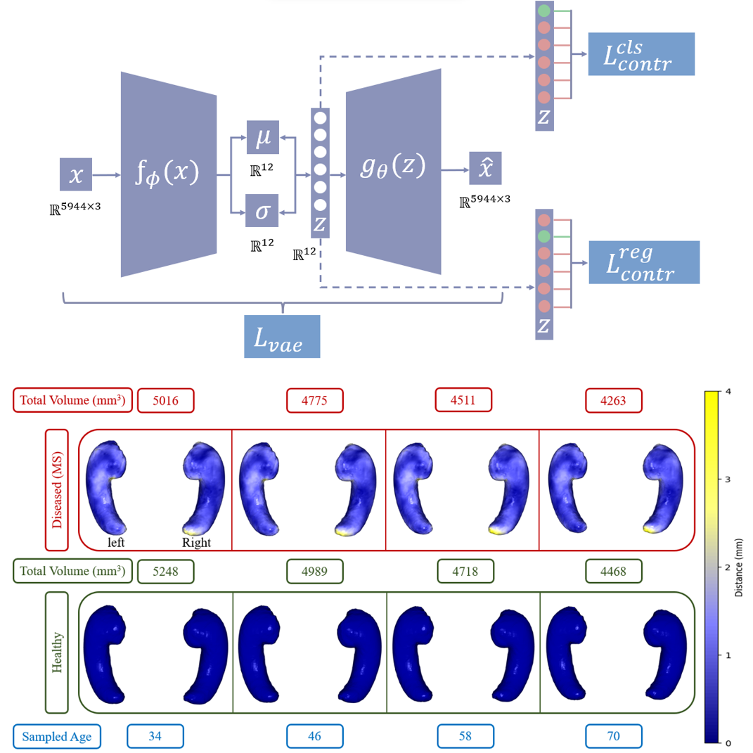
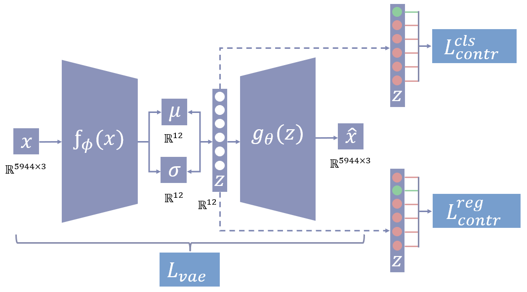
The network’s encoder is based on the SpiralNet++ structure (Gong et al., 2019), where all vertices of an input mesh are interconnected via a spiral trajectory that initiates from a randomly chosen vertex. The execution of spiral convolution operations involves two steps: initially, mesh vertices along the trajectory within a fixed distance are concatenated, a process known as neighborhood aggregation. Following this, the concatenated vertices undergo processing through a multilayer perceptron (MLP) with weight sharing (Kiechle et al., 2023). The decoder module performs a reverse transformation compared to the encoder using the latent space . Our overall network architecture is shown in Figure 1.
Our method uses SpiralNet++ to exploit the local geometric structure of mesh data, preserving spatial relationships between vertices, which is crucial for accurately modeling the hippocampus and torus data. In contrast, we do not use PointNet-type models that focus on global features and may lose critical local geometric information. SpiralNet++ ensures consistent capture of local features through a fixed template, aligning with our goal of disentangling specific factors within hippocampus data (Gong et al., 2019). The importance of maintaining local mesh structure for accurate shape analysis, as highlighted by Litany et al. (Litany et al., 2018), further justifies the use of SpiralNet++ over PointNet-type models.
In the following section, we present the -VAE used for our formulation. Then we discuss supervised guided VAE to explore the excitation-inhibition mechanism. However, we implement the mechanism differently. Finally, in section 2.3, we show the formulation of our method.
2.1 -VAE (Higgins et al., 2016)
Our approach uses the -VAE as the backbone of our network architecture. The VAE uses the Evidence Lower Bound (ELBO) as its objective function, expressed as:
| (1) |
This equation reflects the balance between maximizing the reconstruction accuracy of the model, quantified by the expected log-likelihood of the observed data () given latent variables (), which is , and minimizing the divergence between the posterior distribution of the latent variables under the encoder model and the prior distribution , scaled by the hyperparameter . Here, and are the parameters of the encoder and decoder network. This objective function can be decomposed into two primary components: the reconstruction loss and the Kullback-Leibler divergence, forming the VAE loss demonstrated by the following equations:
| (2) |
where, is the overall -VAE loss consisting of reconstruction and KL divergence loss (multiplied with hyperparameter ).
| (3) |
where, is the input 3D mesh shape and is the reconstructed shape.
| (4) |
where, measures the KL divergence between the posterior () and prior () distributon.
2.2 Supervised Guided VAE (Ding et al., 2020)
The objective function of the supervised guided VAE model is defined as follows:
| (5) |
where is the evidence lower bound, is the excitation loss, and is the inhibition loss calculated using separate feed-forward neural networks. The excitation loss is used to establish a correlation between a specific latent variable, for example, , and a data generative factor like age or scale. The excitation loss is defined as:
| (6) |
where is the latent variable for supervised disentanglement, is the input data, is the label, and parameterizes the excitation network. The inhibition loss is defined as:
| (7) |
In this context, represents a composite of latent variables excluding , and denotes the parameters of the inhibition network. The methodology involves the training of distinct latent variables () to establish correlations with specific features within a dataset (). The inhibition term is designed to avoid unintended associations between other latent variables () and the labeled output. Our approach follows the excitation-inhibition mechanism like the guided VAE but with different losses without the need for separate neural networks.
2.3 Supervised Contrastive VAE (Ours)
We introduce a contrastive loss based on Frosst et al. (2019) applied to the excitation-inhibition mechanism inspired by Ding et al. (2020) and Kiechle et al. (2023) including a threshold hyperparameter in the regression loss for disentangling latent space of a VAE. The loss function is composed of three parts: , , and shown in 8. The first part is the loss function of the VAE, while the other two are the contrastive loss functions.
Contrastive loss learns the representations of the data in the latent space, and our first contrastive loss function enforces the similarity between the samples of the same class and the dissimilarity between the samples of different classes. In our problem setting, classification inherently deals with discrete labels, where the model’s objective is to distinguish between distinct classes. The loss function encourages the latent space to separate data points based on these discrete labels. This loss only applies to the latent variable responsible for the classification task. We use it to disentangle the first latent variable () that correlates with the bump (present or absent) in the torus dataset and disease (healthy or MS) in the hippocampus dataset. Here, the binary labels are represented by . The loss is demonstrated in Figure 1.
| (8) |
| (9) |
In equation 9, the loss function is estimated across the data batch by sampling a neighboring point for each point in the latent space. The likelihood of sampling depends on the distance between points and . The loss is represented by the negative logarithm of the probability of sampling a neighboring point from the same class () as . The temperature parameter regulates the significance assigned to the distances between pairs of points. We implement the inhibition mechanism by introducing a term , weighted by in the denominator of the loss and the formulation ensures that other latent variables from to ( number of latent variables) remain uncorrelated with the classification labels. We use all the values from the other dimensions from the latent space within the exponential term and use in the denominator to take the average. The loss formulation acts like excitation unit when and .
On the other hand, Regression deals with continuous targets in our setting. We employ a threshold parameter (Th) in equation 10 to simulate a classification problem using continuous targets. This is a hyperparameter that controls the granularity of the regression task. It divides the values into separate bins and is completely different from the classification loss function. This loss only applies to the latent variable responsible for the regression task. We formulate the loss function to address our regression problem of disentangling (depicted in figure 1) based on continuous labels such as ages or scales. The loss function categorizes data objects into the same class if their labels fall within a specified range () determined by the threshold.
| (10) |
Overall, we employ the modified soft nearest neighbor losses (SNNL) (Frosst et al., 2019) as part of the inhibition-excitation mechanism, aiming to disentangle specific latent variables associated with distinct data generative factors. Our approach is scalable, allowing extension to more than two latent variables to disentangle additional data-generative factors of interest. While our model can disentangle other latent variables except the targetted ones, it does not enforce supervision for those variables. The SNNL focuses on enhancing latent representations’ quality by promoting similarity among embeddings and assigning probabilities to all samples.
There exists an alternate contrastive loss, InfoNCE (Oord et al., 2018), which is formulated as a binary classification task, distinguishing positive from negative pairs. It compels the model to learn representations where positive pairs are more similar to each other than to negative pairs, effectively maximizing mutual information between positive pairs. However, we opt for a modified SNNL due to its less explicit differentiation between positive and negative pairs, emphasizing the creation of a smoother, probabilistic representation of similarity.
The denominator of our modified SNNL (equation 9 and 10) involves a sum over the exponential terms of all latent representations ( and ) of the samples in the dataset, encompassing both positive and negative samples, and it encourages the model to assign higher probabilities to positive pairs without enforcing a strict binary distinction, as InfoNCE does. Therefore, our model and loss function can address both classification (equation 9) and regression problems (equation 10) using SNNL. The inclusion of an extra term in the denominator, weighted by , enhances the probability of attaining a more disentangled representation. This is achieved by considering all latent representations in the variables not intended for disentanglement for a specific data generative factor.
3 Experiments and Analysis
3.1 Datasets
In this section, we provide an overview of the datasets utilized in this study, namely the hippocampus and synthetic data. All models compared in the results section are assessed using the data from both datasets.
3.1.1 Synthetic Torus Dataset
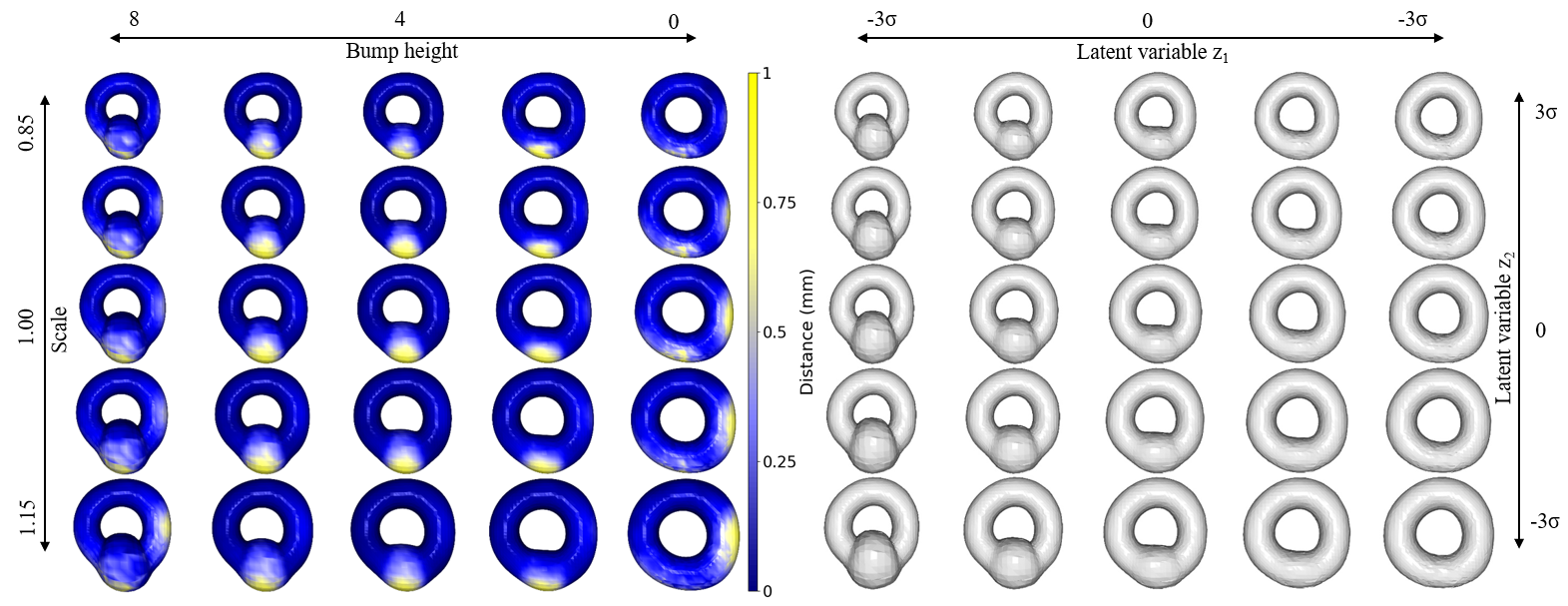
We have a hippocampus dataset that only includes a single scan per subject, it lacks the necessary ground truth to establish the relationship between shape and age. Furthermore, the data only offers scans for healthy and MS populations separately. Longitudinal data, on the other hand, can provide insight into the hippocampal shape of individual subjects over time, taking into account their MS status. Consequently, for evaluation purposes, synthetic data representing a torus with a bump (varying in size and presence/absence) is utilized following the method introduced in an article by Kiechle et al. (2023). We introduce four types of variability (scale of the torus, different noises, presence, and height of the bump) but only two variabilities (bump presence and torus scale) are disentangled in the latent space. We generate 5000 torus data by varying generative factors for our experiments. In figure 2, the color difference illustrates the dissimilarity between original and generated torus shapes, highlighting the variations in torus shapes by adjusting the values of the two latent variables controlling torus bump size and total scale.
3.1.2 Hippocampus Dataset
We utilize a neuroimaging dataset that incorporates diffusion tensor imaging (DTI) scans. The high-resolution data displays a voxel size of 1 mm isotropic, is acquired at 3 Tesla, and consists of volumes measuring 220 × 216 × 20 mm³ (Solar et al., 2021). This dataset encompasses scans from 204 healthy subjects spanning an age range between 32 to 71 years, with 112 females. Additionally, we have scans from subjects with MS (43 subjects aged between 32 to 71, with 35 females and the rest being males) (Valdés Cabrera et al., 2023).
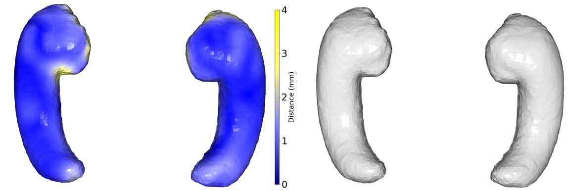
The segmentation of the hippocampus in each scan for healthy subjects is conducted automatically (Efird et al., 2021) and manual segmentation is used for the MS subjects, followed by a series of preprocessing steps. Initially, the volumetric representations (i.e., voxel-based) underwent conversion into 3D mesh representations using a marching cubes algorithm (Lorensen and Cline, 1998). Subsequently, Laplacian surface smoothing and rigid alignment via an iterative closed point algorithm were applied to eliminate rotational artifacts. To ensure uniform topology across instances, Deformetrica (Durrleman et al., 2014) was employed to establish point correspondence across the meshes due to the assumption of meshes having the same topology (Gong et al., 2019). The result of this process is a collection of diffeomorphic deformation maps that illustrate the relationship between a computed mean atlas and the individual subject meshes. Each mesh is characterized by 5944 vertices and 11880 faces. In figure 3, the color difference illustrates the dissimilarity between original and generated hippocampus shapes, and on the right side, original hippocampus data is shown.
3.2 Implementation Details
Our mesh VAE architecture is similar to the SpiralNet++ (Gong et al., 2019). The encoder module comprises four spiral convolution layers with output channel sizes of [8, 8, 8, 8] and a latent channel size of 12. We use latent channel size as a parameter and find that a size of 12 gives the best results in terms of disentanglement. Sizes smaller than 12 reduce reconstruction accuracy, while sizes larger than 12 compromise disentanglement accuracy. We test sizes of 4, 8, 16, 32, and 12 balanced the trade-off most effectively, providing optimal performance for both disentanglement and reconstruction. The decoder module mirrors the transformations of the encoder. We set , according to the parameter tuning results, and employ dilated spiral convolution with subsampling that enhances overall performance. A dilation factor of 2 and a spiral sequence length of 45 are used and those are selected by the parameter tuning process. In the numerical experiments, we adopt an 80/10/10 split for training/validation/testing. The ADAM optimizer is utilized with a batch size of 16, an initial learning rate of , and a training horizon of 300 epochs. We use a scheduler to decay the primary learning rate by a factor of 0.77 every epoch. The proposed contrastive loss functions use temperature and threshold , and all the hyperparameter values are tuned using a hyperparameter optimization framework, Optuna (Akiba et al., 2019). We run all the experiments of models on Nvidia Titan RTX GPUs.
3.3 Evaluation Metrics
In this section, we present the evaluation metrics used to assess the performance of our proposed model. We focus on disentanglement, regression, and classification aspects, employing a variety of metrics suitable for each task.
3.3.1 Separated Attribute Predictability (SAP) (Kumar et al., 2017)
SAP score measures how well the model disentangles different attributes or factors of variation. It quantifies the ability to predict individual attributes from the learned representations. The computation of SAP score involves creating a score matrix, denoted as , of dimensions with latent variables and data generative factors. Each entry in this matrix signifies the linear regression score for predicting the -th factor using solely the -th latent code. The value of the regression, denoted as , represents the predictability. Subsequently, for each column in (corresponding to a factor), the SAP score is determined as follows:
| (11) |
In this equation, is the highest score, is the second highest, and denotes the number of considered factors.
3.3.2 Pearson correlation coefficient (PCC) (Cohen et al., 2009)
We use PCC to calculate the correlation between the values of a specific latent variable and the feature labels (continuous) that the variable is disentangling. The Pearson correlation coefficient, denoted as , quantifies the linear relationship between two continuous variables. It measures how well the data points align along a straight line. The formula for Pearson correlation is as follows:
| (12) |
where is the total number of data points. and represent the values of the two variables for the -th data point. and denote the means of the and values, respectively.
3.3.3 Point Biserial Correlation (PBC)(Brown, 2001)
PBC is used for the correlation between the values of a specific latent variable and the feature labels (binary) that the variable is disentangling. Point biserial correlation measures the association between a binary attribute and a continuous variable and is defined by the following equation:
| (13) |
where and are the means of the continuous variable for positive and negative classes, respectively, is the pooled standard deviation, and are the sample sizes for positive and negative classes and is the total sample size.
3.3.4 Accuracy (Acc.)
Accuracy measures the proportion of correctly classified instances. We use K-nearest neighbor (Imandoust et al., 2013) for accuracy calculation for our classification task. The values of the specific latent variables are used to predict the labels.
3.3.5 Mean Squared Error (MSE)
MSE quantifies the average squared difference between predicted and actual values. The outcomes of K-nearest neighbor (Imandoust et al., 2013) are used for MSE calculation for our regression task. The values of the specific latent variables are used to predict discrete labels.
| (14) |
where is the total data points and and are the original and predicted labels.
3.3.6 Reconstruction Error (Rec. Err.)
Rec. Err. measures the dissimilarity (euclidean distance in 3D) between original and reconstructed 3D mesh shapes.
| (15) |
where is the total data points and and are the original and reconstructed mesh shapes.
3.3.7 1-Nearest Neighbor Accuracy (1-NNA)(Yang et al., 2019)
1-NNA evaluates the quality of learned representations by comparing nearest neighbors in the learned space using Chamfer Distance (CD) and Earth Mover’s Distance (EMD). We calculate 1-NNA accuracy using the 3D coordinates from the original data and the 3D coordinates generated from the decoder of our model. We generate the latent variables from our learned distribution of values from the training set.
Let be the set of generated point clouds, and be the set of reference point clouds with , as the union of and excluding the element , and let represent the nearest neighbor of within . The 1-NN accuracy, denoted as 1-NNA, for the 1-NN classifier is expressed as follows:
| (16) |
where represents the indicator function. In this context, each sample is classified by the 1-NNA classifier as either belonging to or based on the label of its nearest sample. If and are drawn from the same distribution, the accuracy of this classifier should approach 50% with an adequate number of samples. The proximity of the accuracy to 50% reflects the similarity between and , indicating the model’s effectiveness in capturing the target distribution.
CD quantifies the dissimilarity between two point sets by measuring the average distance from each point in one set to its nearest neighbor in the other set. It is defined as follows:
| (17) |
where, and are the two point sets. and represent the cardinalities of sets and , respectively. denotes the Euclidean distance between points and .
EMD, also known as Wasserstein distance, measures the minimum cost required to transform one point distribution into another. It considers the global distribution of points and accounts for both spatial arrangement and quantity. EMD is defined as:
| (18) |
where, represents a transport plan that maps points from set to set . is the cost of transporting point to point .
3.4 Results
In this section, we present a comprehensive evaluation of our proposed model, Supervised Contrastive VAE (SC VAE), using the evaluation metrics discussed in the previous section. The comparison section compares our method with two baselines and two SOTA methods, using synthetic Torus and Hippocampus (containing both healthy and MS subjects) datasets. The comparison is based on disentanglement, correlation, prediction, reconstruction, and data-generative performance. The baseline models are -VAE (Higgins et al., 2016) and -TCVAE (Chen et al., 2018) while we use Supervised Guided VAE (SG VAE) (Ding et al., 2020) and Attribute VAE (Cetin et al., 2023) as SOTA methods.
We provide an ablation study of our method, demonstrating the significance of the inhibition term. Furthermore, we present individual SAP scores for the discrete and continuous labels, when our model is trained to disentangle them separately. Then the training and test time comparisons are shown for all the five models. Lastly, we demonstrate the implementation of our model to analyze 3D hippocampus shape changes due to MS and aging.
3.4.1 Comparison
We compare the models in terms of disentanglement score (SAP), the correlation between the latent variables and labels (Corr.), accuracy (Acc.), and MSE score in predicting the labels from the values of the latent variables using the K-nearest neighbor classifier. The reported SAP scores in table 1 are calculated by averaging the SAP scores for and variables and the models are trained simultaneously for classification and regression tasks for all the scores.
The results, presented in Table 1, include SAP score (average of classification and regression SAP scores), correlation, accuracy, and MSE for all five models across both torus and hippocampus datasets. Our model demonstrates superior performance in SAP scores for both datasets while achieving comparable or better results in terms of correlation, accuracy, and MSE compared to the other models.
| Model | Dataset | SAP | Corr. | Acc. | MSE |
|---|---|---|---|---|---|
| () | () | () | () | ||
| -VAE | Torus | 0.43 | 0.48 | 64.47 | 0.074 |
| Hippocampus | 0.09 | 0.38 | 53.98 | 0.091 | |
| -TCVAE | Torus | 0.45 | 0.48 | 71.95 | 0.071 |
| Hippocampus | 0.11 | 0.39 | 53.23 | 0.093 | |
| SG VAE | Torus | 0.64 | 0.78 | 100 | 0.013 |
| Hippocampus | 0.31 | 0.69 | 98.09 | 0.029 | |
| Attribute VAE | Torus | 0.66 | 0.74 | 100 | 0.017 |
| Hippocampus | 0.32 | 0.66 | 98.13 | 0.028 | |
| SC VAE (Ours) | Torus | 0.69 | 0.75 | 100 | 0.016 |
| Hippocampus | 0.36 | 0.70 | 98.31 | 0.025 |
In Table 2, we present the reconstruction error and 1-NNA scores using CD and EMD for all five models across both datasets. Lower values indicate better performance for both reconstruction and 1-NNA scores. Our model demonstrates superior 1-NNA scores for the torus dataset using EMD. For both datasets, our model’s scores, except for 1-NNA on the torus dataset, are either better or comparable to those of supervised models. However, baseline models exhibit better performance in terms of reconstruction error and the quality of data generation (1-NNA). These results align with expectations, as increased disentanglement in the latent space poses a challenge for models to simultaneously reduce reconstruction error and maintain high-quality data generation capabilities.
To summarize, our proposed method performs better than all four methods in terms of disentanglement, while also showing comparable or better results in terms of prediction and correlation. Additionally, our method performs similarly in terms of reconstruction error and data generation quality when compared to supervised disentangled methods.
| Model | Dataset | Rec. Err. | 1-NNA(%, ) | |
|---|---|---|---|---|
| () | CD | EMD | ||
| -VAE | Torus | 0.25 | 51.37 | 56.25 |
| Hippocampus | 0.85 | 56.58 | 55.96 | |
| -TCVAE | Torus | 0.28 | 52.35 | 54.71 |
| Hippocampus | 0.86 | 56.35 | 55.43 | |
| SG VAE | Torus | 0.33 | 52.78 | 56.33 |
| Hippocampus | 1.08 | 61.79 | 60.05 | |
| Attribute VAE | Torus | 0.36 | 59.38 | 57.81 |
| Hippocampus | 1.09 | 59.38 | 58.37 | |
| SC VAE (Ours) | Torus | 0.38 | 51.56 | 53.12 |
| Hippocampus | 1.07 | 58.69 | 59.76 | |
3.4.2 Ablation Study
Our ablation study shows the significance of the inhibition term using different metrics. In Table 3, we show the ablation study, providing the scores of SAP, correlation, accuracy, MSE, and reconstruction errors for both torus and hippocampus datasets. Introducing the additional denominator term (inhibition when and in equations 9 and 10) results in an increase in SAP score compared to using the SNN loss without any modification (w/o inhibition when and in equations 9 and 10) for both datasets. Meanwhile, the scores of other metrics remain comparable. Here, lower MSE and reconstruction error scores signify improved performance.
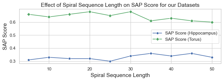
Additionally, we conducted an ablation study to verify the effect of neighborhood information on disentanglement in mesh-based convolutional neural networks. The plot in figure 4 demonstrates that varying the spiral sequence length affects the SAP score for both the hippocampus and torus datasets. The non-linear relationship between spiral length and SAP scores shows that optimal performance occurs at specific lengths, implying that neighborhood connectivity impacts disentanglement. Therefore, the length of the spiral, as neighborhood information, has a significant effect on disentanglement. On a scale of 1, the SAP score varies in the range of 0.07 and 0.06 for the torus and hippocampus data, respectively. The scores would not change much or remain similar if a reasonable spiral length does not affect disentanglement. This justifies our use of SpiralNet++, which leverages such connectivity effectively.
| Model | Dataset | SAP | Corr. | Acc. | MSE | Rec. Err. |
|---|---|---|---|---|---|---|
| () | () | () | () | () | ||
| SC VAE () | Torus | 0.66 | 0.77 | 100 | 0.016 | 0.37 |
| Hippocampus | 0.31 | 0.70 | 98.11 | 0.027 | 1.07 | |
| SC VAE (w/ inhibition) | Torus | 0.68 | 0.75 | 100 | 0.016 | 0.38 |
| Hippocampus | 0.36 | 0.70 | 98.31 | 0.025 | 1.07 |
3.4.3 Training and Test Time
We present the training (seconds per epoch) and test times (seconds per test set) for both the synthetic torus (80% of 5000 instances during training, and 10% each for test and validation) and hippocampus datasets (80% of 553 instances during training, and 10% each for test and validation). Guided VAE exhibits the longest training time due to additional parameters introduced by neural networks for excitation and inhibition mechanisms. Our method requires slightly more time than Attribute VAE during training, while the two baseline methods outperform supervised methods in terms of training time. During test time, our method demonstrates performance comparable to other methods.
| Models | -VAE | -TC- | SG | Attribute | SC | |
| VAE | VAE | VAE | VAE | |||
| (Ours) | ||||||
| Training (Sec./Epoch) | Torus | 6.93 | 7.89 | 23.14 | 9.8 | 10.50 |
| Hippocampus | 0.28 | 0.29 | 0.91 | 0.33 | 0.49 | |
| Test (Sec./Set) | Torus | 0.24 | 0.24 | 0.26 | 0.25 | 0.25 |
| Hippocampus | 0.02 | 0.02 | 0.03 | 0.03 | 0.03 |
3.4.4 SAP Scores for Classification and Regression Tasks
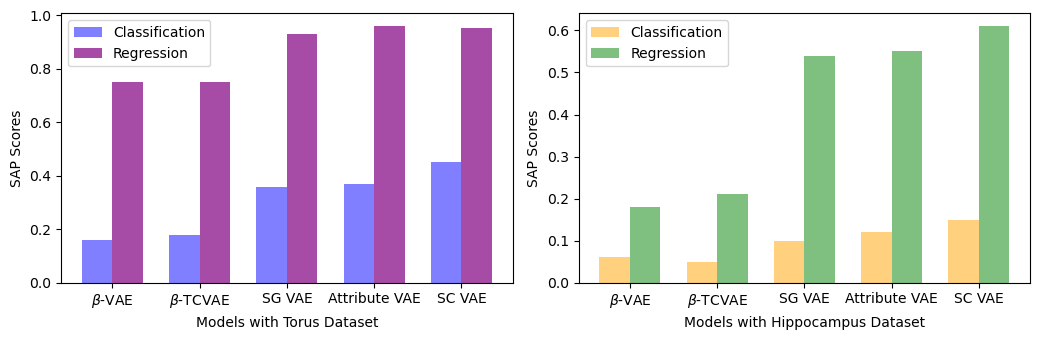
We present the mean SAP score within the comparison section. Figure 5 presents the classification and regression scores for both torus and hippocampus datasets when trained independently (All the other results in different sections were obtained by training classification and regression tasks simultaneously). Our approach demonstrates superior performance in classification and regression tasks for both datasets compared to other methods, except for Attribute VAE, which does a slightly better job in the regression task specifically for the Torus dataset.
3.4.5 MS vs Hippocampal Volume Across Age Groups
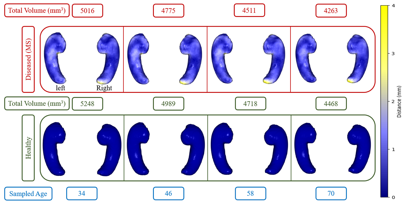
We employ our trained model to produce hippocampus shapes and assess the data-generating capabilities of our model within the domain of medical data. Our trained model demonstrates the ability to capture volume changes according to different data generative factors like age and diseases. By mapping the latent variable values within the range of -3 to +3 onto the age range of MS subjects, we select ages with intervals. Subsequently, we obtain the shapes of the healthy hippocampus by fixing the value at -3 and the MS hippocampus by maintaining the value at 3.
In Figure 6, we present the results for MS vs healthy controls. The lower row displays healthy hippocampus shapes for four sample ages, while the upper row depicts MS hippocampus shapes at those ages. Volume changes (between healthy and MS) are depicted in the first row by the intensity of the blue color and yellow represents the highest change in millimeters. The figure illustrates a noticeable decrease in hippocampus size with advancing age, particularly affecting the right hippocampus in MS. The tail of the right hippocampus has more atrophy than other regions.
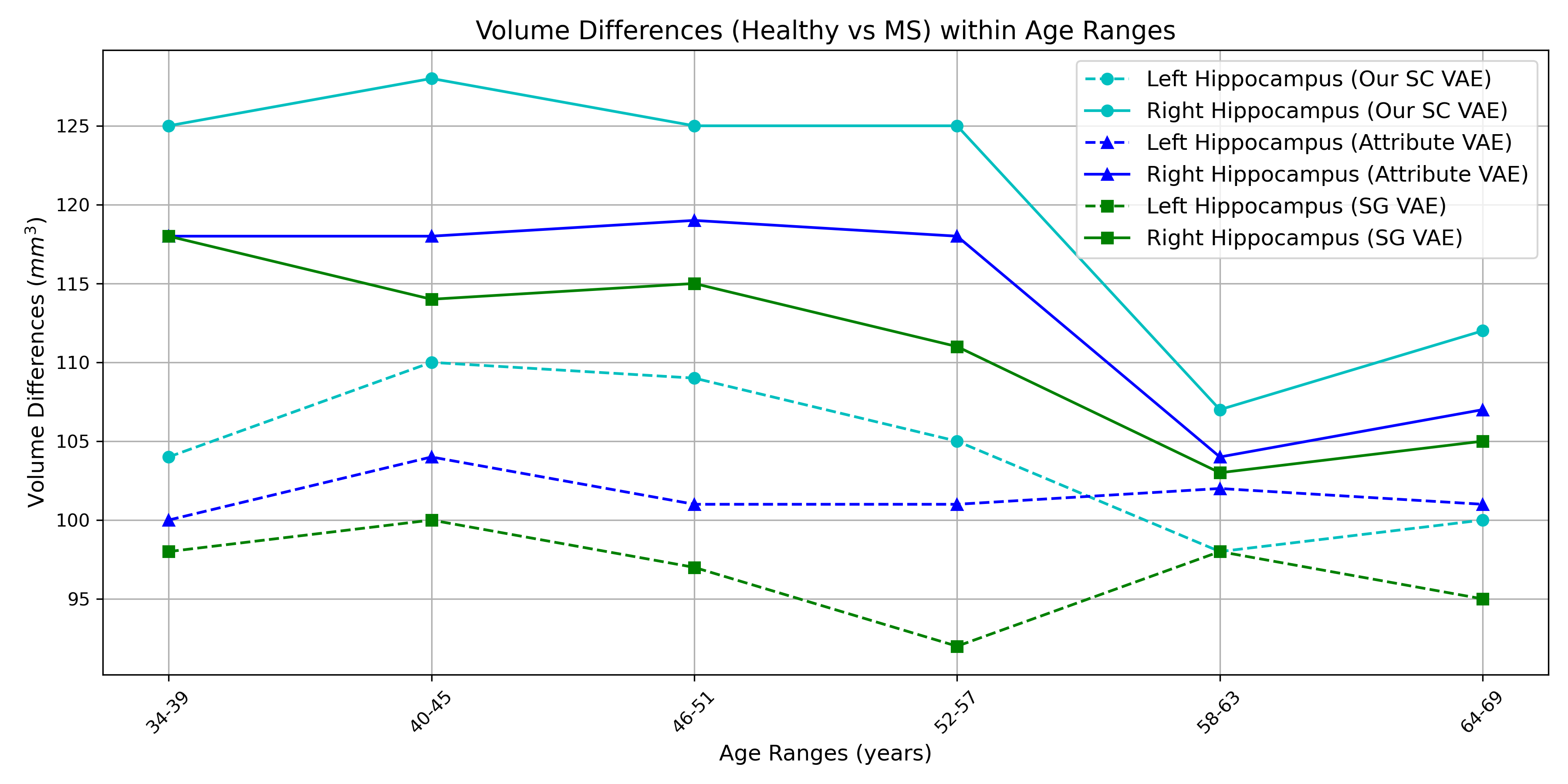
Our findings align with previous research by Roosendaal et al. (2010) and Hulst et al. (2015), which reported a larger reduction in the volume of the right hippocampus compared to the left hippocampus due to MS. Additionally, the overall hippocampus volume is lower in the MS population according to our results and the reduction of volume is also reported in the findings of Valdés Cabrera et al. (2023). However, the volume reduction (4.5%) by our method is lower than Valdés Cabrera et al. (2023) (9%) who used DTI for calculating volumes, and it is expected because our classification (presence or absence of MS) SAP score is lower than the regression (age) SAP score. Therefore, we need more data for the MS population for more accurate results. We also show volume differences in Figure 7 for the three supervised disentangled methods (SG VAE, Attribute VAE, and our SC VAE) and our method shows the highest volume difference, which is closer (compared to other methods) to the average trend found in (Valdés Cabrera et al., 2023). Additionally, we conducted a one-sample t-test (Chorin et al., 2020) to examine whether there was a significant difference in hippocampal volume between healthy and MS populations, and we found the differences are significant (). In Figure 7, the plot illustrates the greater decrease in the volume of the right hippocampus compared to the left hippocampus in patients with MS. We generate the plot by generating 10 shapes (using the three models) from each range, calculating the volume and then take the average volume.
4 Discussion and Conclusion
4.1 Discussion
Our study contributes to the field of medical imaging and shape analysis in several ways. The proposed method enhances disentanglement performance for categorical and continuous labels in the context of 3D mesh data. The analysis of anatomical shape variations across various factors, including age and disease (MS), through the generation of 3D shapes, provides valuable insights into the relationship between neurological disorders and hippocampal shape changes.
Despite the promising results, there are limitations to our approach. The generalization of our model to diverse populations and datasets needs further exploration. We also need to improve the disentanglement performance of disease status for better prediction and reconstruction. Additionally, the mesh convolution technique we used, as outlined by Gong et al. (2019), necessitates the registration of meshes to a template mesh. Consequently, it is crucial to investigate methods that do not rely on assumptions about mesh topology for the analysis of complex shapes. Also, Our classification and regression losses are mostly similar, with only minor differences. Therefore, a unified formulation could be utilized to compactly represent the loss function. Future work would involve the incorporation of longitudinal data and exploration of the generalizability of the proposed method.
4.2 Conclusion
In this paper, we propose a novel approach for disentangling 3D mesh shape (hippocampal or synthetic) variations from DTI or synthetic datasets and applied in the context of neurological disorders. Our method, which uses a Mesh VAE enhanced with Supervised Contrastive Learning, exhibits superior disentanglement capabilities, particularly in identifying age and disease status in patients with MS. Additionally, our method demonstrates comparable or better performance in all other metrics. The validity of our method is also demonstrated by a synthetic torus dataset.
We aim to extract meaningful representations of anatomical structures, providing insights into the complexities of diseases and age-related variations in the hippocampus by integrating novel and efficient latent space disentanglement techniques. Our method demonstrates the extraction of valuable insights into hippocampal morphology and atrophy linked to age and MS, even in the face of challenges posed by the absence of longitudinal data in limited datasets.
Acknowledgments
Operating grant was provided by the Canadian Institutes of Health Research (CIHR) and the DTI dataset acquisition was funded by the University Hospital Foundation and the Women and Children’s Health Research Institute. Author DC acknowledges student funding from Natural Sciences and Engineering Research Council DG program. Author CB acknowledges funding by CIHR and Canada Research Chairs. Infrastructure was provided by the Canada Foundation for Innovation, Alberta Innovation and Advanced Education, and the University Hospital Foundation.
Ethical Standards
No ethics approval was required for the synthetic data analysis. The neuroimaging study was approved by the Human Research Ethics Board at the University of Alberta
Conflicts of Interest
We declare we don’t have conflicts of interest.
Data availability
The GitHub repository contains the script for generating synthetic data. Although the hippocampus data is confidential and cannot be shared, the preprocessing scripts are provided and can be utilized for any publicly available MRI data that includes hippocampus segmentation.
References
- Akiba et al. (2019) Takuya Akiba, Shotaro Sano, Toshihiko Yanase, Takeru Ohta, and Masanori Koyama. Optuna: A next-generation hyperparameter optimization framework. In Proceedings of the 25th ACM SIGKDD international conference on knowledge discovery & data mining, pages 2623–2631, 2019.
- Altaf et al. (2019) Fouzia Altaf, Syed MS Islam, Naveed Akhtar, and Naeem Khalid Janjua. Going deep in medical image analysis: concepts, methods, challenges, and future directions. IEEE Access, 7:99540–99572, 2019.
- Aneja et al. (2021) Jyoti Aneja, Alex Schwing, Jan Kautz, and Arash Vahdat. A contrastive learning approach for training variational autoencoder priors. Advances in neural information processing systems, 34:480–493, 2021.
- Brown (2001) James Dean Brown. Point-biserial correlation coefficients. Statistics, 5(3):12–6, 2001.
- Burgess et al. (2018) Christopher P Burgess, Irina Higgins, Arka Pal, Loic Matthey, Nick Watters, Guillaume Desjardins, and Alexander Lerchner. Understanding disentangling in -vae. arXiv preprint arXiv:1804.03599, 2018.
- Cetin et al. (2023) Irem Cetin, Maialen Stephens, Oscar Camara, and Miguel A González Ballester. Attri-vae: Attribute-based interpretable representations of medical images with variational autoencoders. Computerized Medical Imaging and Graphics, 104:102158, 2023.
- Chen et al. (2018) Ricky TQ Chen, Xuechen Li, Roger B Grosse, and David K Duvenaud. Isolating sources of disentanglement in variational autoencoders. Advances in neural information processing systems, 31, 2018.
- Chorin et al. (2020) Ehud Chorin, Matthew Dai, Eric Shulman, Lalit Wadhwani, Roi Bar-Cohen, Chirag Barbhaiya, Anthony Aizer, Douglas Holmes, Scott Bernstein, Michael Spinelli, et al. The qt interval in patients with covid-19 treated with hydroxychloroquine and azithromycin. Nature medicine, 26(6):808–809, 2020.
- Cohen et al. (2009) Israel Cohen, Yiteng Huang, Jingdong Chen, Jacob Benesty, Jacob Benesty, Jingdong Chen, Yiteng Huang, and Israel Cohen. Pearson correlation coefficient. Noise reduction in speech processing, pages 1–4, 2009.
- Deng et al. (2020) Yu Deng, Jiaolong Yang, Dong Chen, Fang Wen, and Xin Tong. Disentangled and controllable face image generation via 3d imitative-contrastive learning. In Proceedings of the IEEE/CVF conference on computer vision and pattern recognition, pages 5154–5163, 2020.
- Ding et al. (2020) Zheng Ding, Yifan Xu, Weijian Xu, Gaurav Parmar, Yang Yang, Max Welling, and Zhuowen Tu. Guided variational autoencoder for disentanglement learning. In Proceedings of the IEEE/CVF conference on computer vision and pattern recognition, pages 7920–7929, 2020.
- Dupont (2018) Emilien Dupont. Learning disentangled joint continuous and discrete representations. Advances in neural information processing systems, 31, 2018.
- Durrleman et al. (2014) Stanley Durrleman, Marcel Prastawa, Nicolas Charon, Julie R Korenberg, Sarang Joshi, Guido Gerig, and Alain Trouvé. Morphometry of anatomical shape complexes with dense deformations and sparse parameters. NeuroImage, 101:35–49, 2014.
- Efird et al. (2021) Cory Efird, Samuel Neumann, Kevin G Solar, Christian Beaulieu, and Dana Cobzas. Hippocampus segmentation on high resolution diffusion mri. In 2021 IEEE 18th International Symposium on Biomedical Imaging (ISBI), pages 1369–1372. IEEE, 2021.
- Estermann and Wattenhofer (2023) Benjamin Estermann and Roger Wattenhofer. Dava: Disentangling adversarial variational autoencoder. arXiv preprint arXiv:2303.01384, 2023.
- Foti et al. (2022) Simone Foti, Bongjin Koo, Danail Stoyanov, and Matthew J Clarkson. 3d shape variational autoencoder latent disentanglement via mini-batch feature swapping for bodies and faces. In Proceedings of the IEEE/CVF conference on computer vision and pattern recognition, pages 18730–18739, 2022.
- Frosst et al. (2019) Nicholas Frosst, Nicolas Papernot, and Geoffrey Hinton. Analyzing and improving representations with the soft nearest neighbor loss. In International conference on machine learning, pages 2012–2020. PMLR, 2019.
- Gong et al. (2019) Shunwang Gong, Lei Chen, Michael Bronstein, and Stefanos Zafeiriou. Spiralnet++: A fast and highly efficient mesh convolution operator. In Proceedings of the IEEE/CVF international conference on computer vision workshops, pages 0–0, 2019.
- Higgins et al. (2016) Irina Higgins, Loic Matthey, Arka Pal, Christopher Burgess, Xavier Glorot, Matthew Botvinick, Shakir Mohamed, and Alexander Lerchner. beta-vae: Learning basic visual concepts with a constrained variational framework. In International conference on learning representations, 2016.
- Huang et al. (2023) Zhicheng Huang, Xiaojie Jin, Chengze Lu, Qibin Hou, Ming-Ming Cheng, Dongmei Fu, Xiaohui Shen, and Jiashi Feng. Contrastive masked autoencoders are stronger vision learners. IEEE Transactions on Pattern Analysis and Machine Intelligence, 2023.
- Hulst et al. (2015) Hanneke E Hulst, Menno M Schoonheim, Quinten Van Geest, Bernard MJ Uitdehaag, Frederik Barkhof, and Jeroen JG Geurts. Memory impairment in multiple sclerosis: relevance of hippocampal activation and hippocampal connectivity. Multiple Sclerosis Journal, 21(13):1705–1712, 2015.
- Imandoust et al. (2013) Sadegh Bafandeh Imandoust, Mohammad Bolandraftar, et al. Application of k-nearest neighbor (knn) approach for predicting economic events: Theoretical background. International journal of engineering research and applications, 3(5):605–610, 2013.
- Kiechle et al. (2023) Johannes Kiechle, Dylan Miller, Jordan Slessor, Matthew Pietrosanu, Linglong Kong, Christian Beaulieu, and Dana Cobzas. Explaining anatomical shape variability: Supervised disentangling with a variational graph autoencoder. In 2023 IEEE 20th International Symposium on Biomedical Imaging (ISBI), pages 1–5. IEEE, 2023.
- Kim and Mnih (2018) Hyunjik Kim and Andriy Mnih. Disentangling by factorising. In International Conference on Machine Learning, pages 2649–2658. PMLR, 2018.
- Kingma et al. (2019) Diederik P Kingma, Max Welling, et al. An introduction to variational autoencoders. Foundations and Trends® in Machine Learning, 12(4):307–392, 2019.
- Kipf and Welling (2016) Thomas N Kipf and Max Welling. Variational graph auto-encoders. arXiv preprint arXiv:1611.07308, 2016.
- Kumar et al. (2017) Abhishek Kumar, Prasanna Sattigeri, and Avinash Balakrishnan. Variational inference of disentangled latent concepts from unlabeled observations. arXiv preprint arXiv:1711.00848, 2017.
- Litany et al. (2018) Or Litany, Alex Bronstein, Michael Bronstein, and Ameesh Makadia. Deformable shape completion with graph convolutional autoencoders. In Proceedings of the IEEE conference on computer vision and pattern recognition, pages 1886–1895, 2018.
- Lorensen and Cline (1998) William E Lorensen and Harvey E Cline. Marching cubes: A high resolution 3d surface construction algorithm. In Seminal graphics: pioneering efforts that shaped the field, pages 347–353. 1998.
- Lv et al. (2021) Chenlei Lv, Weisi Lin, and Baoquan Zhao. Voxel structure-based mesh reconstruction from a 3d point cloud. IEEE Transactions on Multimedia, 24:1815–1829, 2021.
- Oord et al. (2018) Aaron van den Oord, Yazhe Li, and Oriol Vinyals. Representation learning with contrastive predictive coding. arXiv preprint arXiv:1807.03748, 2018.
- Pan et al. (2018) Shirui Pan, Ruiqi Hu, Guodong Long, Jing Jiang, Lina Yao, and Chengqi Zhang. Adversarially regularized graph autoencoder for graph embedding. arXiv preprint arXiv:1802.04407, 2018.
- Roosendaal et al. (2010) Stefan D Roosendaal, Hanneke E Hulst, Hugo Vrenken, Heleen EM Feenstra, Jonas A Castelijns, Petra JW Pouwels, Frederik Barkhof, and Jeroen JG Geurts. Structural and functional hippocampal changes in multiple sclerosis patients with intact memory function. Radiology, 255(2):595–604, 2010.
- Solar et al. (2021) Kevin Grant Solar, Sarah Treit, and Christian Beaulieu. High resolution diffusion tensor imaging of the hippocampus across the healthy lifespan. Hippocampus, 31(12):1271–1284, 2021.
- Sun et al. (2022) Hao Sun, Nick Pears, and Yajie Gu. Information bottlenecked variational autoencoder for disentangled 3d facial expression modelling. In Proceedings of the IEEE/CVF Winter Conference on Applications of Computer Vision, pages 157–166, 2022.
- Valdés Cabrera et al. (2023) Diana Valdés Cabrera, Gregg Blevins, Penelope Smyth, Derek Emery, Kevin Grant Solar, and Christian Beaulieu. High-resolution diffusion tensor imaging and t2 mapping detect regional changes within the hippocampus in multiple sclerosis. NMR in Biomedicine, 36(9):e4952, 2023.
- Van der Velden et al. (2022) Bas HM Van der Velden, Hugo J Kuijf, Kenneth GA Gilhuijs, and Max A Viergever. Explainable artificial intelligence (xai) in deep learning-based medical image analysis. Medical Image Analysis, 79:102470, 2022.
- Wang et al. (2017) Chun Wang, Shirui Pan, Guodong Long, Xingquan Zhu, and Jing Jiang. Mgae: Marginalized graph autoencoder for graph clustering. In Proceedings of the 2017 ACM on Conference on Information and Knowledge Management, pages 889–898, 2017.
- Yang et al. (2019) Guandao Yang, Xun Huang, Zekun Hao, Ming-Yu Liu, Serge Belongie, and Bharath Hariharan. Pointflow: 3d point cloud generation with continuous normalizing flows. In Proceedings of the IEEE/CVF international conference on computer vision, pages 4541–4550, 2019.